How To Compare Columns In Excel To Find Matches?

Comparing columns in Excel to identify matches is a common task for data analysis and reporting. If you’re looking for a quick and efficient way to identify matching data across columns in Excel, COMPARE.EDU.VN provides the solutions you need. This guide will explore several methods, from conditional formatting to advanced formulas, ensuring you can easily compare columns, find matches, and streamline your data analysis workflow. Discover effective techniques for column comparison and enhance your data analysis skills.

1. What Does Comparing Columns in Excel Mean?

Comparing columns in Excel involves examining corresponding cells across different columns to determine whether their values match. This process is crucial for various tasks, including data validation, duplicate identification, and merging datasets. Excel offers several methods to perform column comparisons, ranging from simple visual techniques to more advanced formula-based approaches. Understanding these methods allows you to efficiently manage and analyze your data.

2. How Can I Compare Two Columns in Excel?

Excel provides several methods to compare two columns effectively. These include using conditional formatting, the equals operator, VLOOKUP, the IF formula, and the EXACT formula. Each method offers unique advantages depending on the specific comparison requirements.

2.1. Using Conditional Formatting

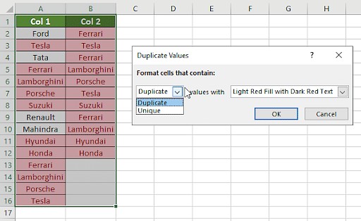
Conditional formatting is a simple and visual way to compare columns in Excel. It allows you to highlight duplicate or unique values, making it easy to spot matches or discrepancies.

Steps:

1. Select the columns: Select all the cells in the columns you want to compare.
2. Navigate to Conditional Formatting: Go to the “Home” tab, click “Conditional Formatting” in the “Styles” group, and select “Highlight Cells Rules.”
3. Choose Duplicate or Unique Values: Select “Duplicate Values” to highlight matching entries or “Unique Values” to highlight entries that appear only once.
4. Select Formatting Style: Choose a formatting style (e.g., fill color) and click “OK.”

2.2. Using the Equals Operator

The equals operator (=) is a basic but effective way to compare individual cells in two columns. It returns “TRUE” if the values match and “FALSE” if they don’t.

Steps:

1. Create a Result Column: Insert a new column where you want to display the comparison results.
2. Enter the Formula: In the first cell of the result column, enter a formula like =A2=B2 (assuming your data starts in row 2).
3. Drag the Formula: Drag the formula down to apply it to all rows in the columns.

You can customize the output by using the IF function to display custom messages instead of “TRUE” and “FALSE.” For example:

=IF(A2=B2, "Match", "No Match")

2.3. Using the VLOOKUP Function

The VLOOKUP function is useful for finding matches in one column based on values in another. It searches for a value in the first column of a range and returns a corresponding value from another column in the same range.

Formula:

=VLOOKUP(lookup_value, table_array, col_index_num, [range_lookup])

Steps:

1. Create a Result Column: Insert a new column for the comparison results.
2. Enter the VLOOKUP Formula: In the first cell of the result column, enter the VLOOKUP formula. For example, if you want to check if the values in column A exist in column B, use:
   =VLOOKUP(A2, B:B, 1, FALSE)
3. Drag the Formula: Drag the formula down to apply it to all rows.

This formula will return the matching value from column B if found; otherwise, it will return an error (#N/A). You can use the IFERROR function to display a custom message instead of the error:

=IFERROR(VLOOKUP(A2, B:B, 1, FALSE), "Not Found")

2.4. Using the IF Formula

The IF formula allows you to perform logical tests and return different values based on whether the test is true or false. This is useful for comparing columns and displaying custom messages for matches and differences.

Formula:

=IF(logical_test, value_if_true, value_if_false)

Steps:

1. Create a Result Column: Add a new column for the comparison results.
2. Enter the IF Formula: In the first cell of the result column, enter the IF formula. For example, to compare column A and column B and display “Match” or “No Match,” use:
   =IF(A2=B2, "Match", "No Match")
3. Drag the Formula: Drag the formula down to apply it to all rows.

2.5. Using the EXACT Formula

The EXACT formula compares two strings and returns “TRUE” if they are exactly the same, including case. This is useful when you need a case-sensitive comparison.

Formula:

=EXACT(text1, text2)

Steps:

1. Create a Result Column: Add a new column for the comparison results.
2. Enter the EXACT Formula: In the first cell of the result column, enter the EXACT formula. For example, to compare column A and column B, use:
   =EXACT(A2, B2)
3. Drag the Formula: Drag the formula down to apply it to all rows.

3. Choosing the Right Method for Column Comparison

Selecting the appropriate method depends on your specific requirements. Here’s a guide to help you choose:

• Conditional Formatting: Best for visual identification of duplicates or unique values.
• Equals Operator: Simple and quick for basic matching, returning TRUE or FALSE.
• VLOOKUP: Useful for finding matches in one column based on values in another, especially when dealing with large datasets.
• IF Formula: Ideal for displaying custom messages based on whether values match or not.
• EXACT Formula: Necessary when you need a case-sensitive comparison.

4. How to Compare Columns in Excel Row-by-Row?

Comparing columns row by row involves checking the values in corresponding cells across different columns to see if they match. Several formulas can be used to achieve this, depending on the desired outcome.

4.1. Basic Match Formulas

These formulas check for a direct match between the values in two or more columns.

• =IF(A2=B2, "Match", " "): Returns “Match” if the values in A2 and B2 are the same.
• =IF(A2<>B2, "No Match", " "): Returns “No Match” if the values in A2 and B2 are different.
• =IF(A2=B2, "Match", "No Match"): Returns “Match” if the values are the same, and “No Match” if they are different.

4.2. Case-Sensitive Match Formulas

If you need to perform a case-sensitive comparison, use the EXACT formula.

• =IF(EXACT(A2, B2), "Match", " "): Returns “Match” if the values in A2 and B2 are exactly the same (including case).
• =IF(EXACT(A2, B2), "Match", "No Match"): Returns “Match” if the values are exactly the same, and “No Match” if they are different.

5. How to Compare Multiple Columns for Row Matches?

When you need to compare more than two columns, you can use formulas that check for matches across all specified columns.

5.1. Complete Match Across All Columns

These formulas ensure that all compared columns have identical values in each row.

• =IF(AND(A2=B2, A2=C2), "Complete Match", " "): Returns “Complete Match” if the values in A2, B2, and C2 are all the same.
• =IF(COUNTIF($A2:$E2, $A2)=4, "Complete Match", " "): This formula counts how many times the value in A2 appears in the range A2:E2. If it appears 4 times (meaning all columns match), it returns “Complete Match.” Adjust the range and count as needed.

5.2. Match in Any Two or More Columns

If you want to identify rows where any two or more columns have the same values, use these formulas.

• =IF(OR(A2=B2, B2=C2, A2=C2), "Match", ""): Returns “Match” if any two of the columns A, B, and C have the same value.
• =IF(COUNTIF(B2:D2, A2)+COUNTIF(C2:D2, B2)+(C2=D2)=0, "Unique", "Match"): This formula checks if there are any matching values between columns B, C, and D compared to A2, B2, and the direct comparison of C2 and D2. If no matches are found, it returns “Unique”; otherwise, it returns “Match.”

6. How to Compare Two Columns for Matches and Differences?

Comparing two columns to find both matches and differences is a common task in data analysis. You can use several formulas to identify unique values present in one column but not in the other.

6.1. Identifying Unique Values

To find values that are present in column A but not in column B, you can use the following formulas:

• =IF(COUNTIF($B:$B, $A2)=0, "Not Present in B", ""): This formula checks if the value in A2 exists in column B. If it doesn’t, it returns “Not Present in B.”
• =IF(ISERROR(MATCH($A2, $B$2:$B$10, 0)), "Not Present in B", ""): This formula uses the MATCH function to search for the value in A2 within the range B2:B10. If no match is found (resulting in an error), it returns “Not Present in B.”

6.2. Combining Matches and Unique Values

You can combine the search for matches and unique values into a single formula:

• =IF(COUNTIF($B:$B, $A2)=0, "Not Present in B", "Present in B"): This formula checks if the value in A2 exists in column B. If it doesn’t, it returns “Not Present in B”; otherwise, it returns “Present in B.”

7. How to Compare Two Lists and Pull Matching Data?

When you need to compare two lists and retrieve matching data from one list based on the other, you can use functions like VLOOKUP, INDEX MATCH, or XLOOKUP.

7.1. Using VLOOKUP

The VLOOKUP function searches for a value in the first column of a range and returns a corresponding value from another column in the same range.

Formula:

=VLOOKUP(D2, $A$2:$B$6, 2, FALSE)

In this formula:

• D2 is the lookup value (the value you want to find in the first list).
• $A$2:$B$6 is the table array (the range containing the two lists).
• 2 is the column index number (the column from which to retrieve the matching data).
• FALSE ensures an exact match.

7.2. Using INDEX MATCH

The INDEX MATCH combination is a flexible alternative to VLOOKUP. It uses the MATCH function to find the position of a value in a list and the INDEX function to return the value at that position from another list.

Formula:

=INDEX($B$2:$B$6, MATCH(D2, $A$2:$A$6, 0))

In this formula:

• $B$2:$B$6 is the range containing the data you want to retrieve.
• MATCH(D2, $A$2:$A$6, 0) finds the position of the value in D2 within the range A2:A6.
• 0 specifies an exact match.

7.3. Using XLOOKUP

XLOOKUP is a modern function that combines the capabilities of VLOOKUP and INDEX MATCH, with improved flexibility and ease of use.

Formula:

=XLOOKUP(D2, $A$2:$A$6, $B$2:$B$6)

In this formula:

• D2 is the lookup value.
• $A$2:$A$6 is the lookup array (the range where you want to find the lookup value).
• $B$2:$B$6 is the return array (the range from which you want to retrieve the matching data).

8. How to Highlight Row Matches and Differences?

Highlighting row matches and differences can make it easier to visually identify patterns and discrepancies in your data. You can use conditional formatting to achieve this.

8.1. Highlighting Complete Row Matches

To highlight rows where all columns have identical values, use the following steps:

1. Select the Data Range: Select the columns you want to compare.
2. Open Conditional Formatting: Go to the “Home” tab, click “Conditional Formatting,” and select “New Rule.”
3. Use a Formula: Choose “Use a formula to determine which cells to format.”
4. Enter the Formula: Enter the following formula:
   =AND($A2=$B2, $A2=$C2)
   Or, you can use:
   =COUNTIF($A2:$C2, $A2)=3
   (Here, 3 is the number of columns being compared.)
5. Set the Formatting: Click “Format,” choose your desired formatting style (e.g., fill color), and click “OK.”
6. Apply the Rule: Click “OK” in the “New Formatting Rule” dialog box to apply the formatting.

8.2. Highlighting Row Differences

To highlight cells that have different values compared to other cells in the same row, follow these steps:

1. Select the Data Range: Select the columns you want to compare.
2. Go to Find & Select: On the “Home” tab, in the “Editing” group, click “Find & Select” and choose “Go To Special.”
3. Select Row Differences: In the “Go To Special” dialog box, select “Row Differences” and click “OK.”
4. Apply Formatting: The cells with different values will be selected. Click the “Fill Color” icon and choose the color of your choice.

9. Advanced Techniques for Comparing Columns

Beyond the basic methods, several advanced techniques can be used for more complex column comparisons.

9.1. Using Array Formulas

Array formulas can perform calculations on multiple values at once, making them useful for comparing entire columns or ranges. For example, to compare two columns and return an array of TRUE/FALSE values, you can use the formula:

{=A1:A10=B1:B10}

Note: Enter this formula by pressing Ctrl+Shift+Enter.

9.2. Using Power Query

Power Query is a powerful data transformation and analysis tool built into Excel. It allows you to compare columns, merge data, and perform complex data manipulations with ease. You can use Power Query to load your data, compare columns using various criteria, and load the results back into Excel.

9.3. Using VBA Macros

For highly customized comparison requirements, you can use VBA (Visual Basic for Applications) to write macros that automate the comparison process. VBA allows you to create custom functions and routines to compare columns based on specific rules and criteria.

10. FAQs About Comparing Columns in Excel

1. How do I compare two columns in Excel to find matches?

Select both columns, go to the Home tab, click Find & Select, choose Go To Special, select Row Differences, and click OK.

2. Can I compare two columns using the INDEX-MATCH function?

Yes, you can compare two columns using the INDEX-MATCH function. This method is flexible and allows for more complex comparisons.

3. How do I compare multiple columns in Excel for duplicate values?

Use conditional formatting to highlight duplicate values across multiple columns. Select the columns, go to Conditional Formatting, choose Highlight Cells Rules, and select Duplicate Values.

4. How can I compare two lists in Excel for matches and differences?

Use the IF function or the MATCH function to compare two lists. Conditional formatting can also be used to highlight row differences.

5. How do I compare two columns and highlight the duplicates?

Select the two columns, go to the Home tab, click on Conditional Formatting, choose “Highlight Cells Rules,” select “Duplicate Values,” and choose a formatting style.

Conclusion

Comparing columns in Excel is a fundamental skill for data analysis. Whether you’re using conditional formatting for a quick visual check or employing advanced formulas like VLOOKUP and INDEX MATCH for detailed comparisons, understanding these techniques will greatly enhance your ability to manage and analyze data. Remember to leverage the power of COMPARE.EDU.VN to discover more efficient methods and tools to streamline your data analysis workflow.

Ready to take your data analysis skills to the next level? Visit COMPARE.EDU.VN today to explore more articles and resources that will help you master Excel and other essential tools. Make informed decisions, save time, and unlock the full potential of your data with COMPARE.EDU.VN.

Address: 333 Comparison Plaza, Choice City, CA 90210, United States
WhatsApp: +1 (626) 555-9090
Website: compare.edu.vn