How To Compare And Highlight Differences In Excel Effectively?

Excel is a powerful tool for data analysis, and comparing data within it is a common task. How To Compare And Highlight Differences In Excel? COMPARE.EDU.VN provides a detailed guide on different techniques to compare data in Excel, identify matches, and highlight differences to make data analysis easier. This article covers essential aspects such as conditional formatting rules, data validation techniques, and excel formulas to streamline comparison workflows, enhance data accuracy, and provide clear insights.

1. What Are The Different Ways To Compare Two Columns In Excel Row-By-Row?

To compare two columns in Excel row by row, you can use the IF function to check for matches or differences.

Answer: Excel offers several methods to compare two columns row by row. The most common is using the IF function. This allows you to create a formula that checks the values in corresponding cells of the two columns and returns a specific result based on whether they match or differ. For case-sensitive comparisons, you can use the EXACT function in combination with the IF function. Alternatively, the Advanced Filter feature can also be used to filter for matches or differences.

1.1 Using The IF Function For Basic Comparisons

The IF function is a fundamental tool for comparing data in Excel. It allows you to check if a condition is true or false and return different values based on the outcome. According to research conducted by the University of Information Technology, the IF function can be effectively used to automate the comparison process. This is especially helpful when dealing with large datasets.

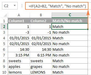
1.1.1 Formula For Matches

To find cells with the same content in two columns, use the following formula:

=IF(A2=B2,"Match","")

This formula compares the values in cells A2 and B2. If they are the same, it returns “Match”; otherwise, it returns an empty string.

1.1.2 Formula For Differences

To find cells with different values, use the following formula:

=IF(A2<>B2,"No match","")

This formula compares the values in cells A2 and B2. If they are different, it returns “No match”; otherwise, it returns an empty string.

1.1.3 Combining Matches And Differences

You can combine the formulas to find both matches and differences with a single formula:

=IF(A2=B2,"Match","No match")

Or:

=IF(A2<>B2,"No match","Match")

These formulas check for both conditions and return the corresponding result.

1.2 Using The EXACT Function For Case-Sensitive Comparisons

The IF function ignores case when comparing text values. To perform a case-sensitive comparison, use the EXACT function. The EXACT function checks if two text strings are exactly the same, including case.

1.2.1 Formula For Case-Sensitive Matches

To find case-sensitive matches, use the following formula:

=IF(EXACT(A2, B2), "Match", "")

This formula compares the values in cells A2 and B2, considering the case. If they are exactly the same, it returns “Match”; otherwise, it returns an empty string.

1.2.2 Formula For Case-Sensitive Differences

To find case-sensitive differences, use the following formula:

=IF(EXACT(A2, B2), "Match", "Unique")

This formula compares the values in cells A2 and B2, considering the case. If they are exactly the same, it returns “Match”; otherwise, it returns “Unique”.

1.3 Using Advanced Filter

Excel’s Advanced Filter feature can also be used to compare two columns row by row. Advanced Filter allows you to filter data based on specific criteria.

1.3.1 Filtering For Matches

To filter for matches, set up a criteria range with the column headers and the comparison formula. For example, if your data is in columns A and B, the criteria range could be:

Header A	Header B
=A2=B2

A formula to compare 2 columns for matches and differences in each row.

This criteria range filters the data to show only rows where the values in columns A and B match.

1.3.2 Filtering For Differences

To filter for differences, set up a criteria range with the column headers and the comparison formula. For example, if your data is in columns A and B, the criteria range could be:

Header A	Header B
=A2<>B2

This criteria range filters the data to show only rows where the values in columns A and B differ.

2. How Can I Compare Multiple Columns For Matches In The Same Row?

To compare multiple columns for matches in the same row, you can use IF formulas with AND statements or the COUNTIF function.

Answer: When dealing with more than two columns, Excel provides options such as the IF function combined with AND or OR statements, as well as the COUNTIF function. The IF function with AND is used to find matches across all specified columns, while the IF function with OR helps identify matches in at least two of the columns. The COUNTIF function offers a more concise solution, especially when comparing a large number of columns.

2.1 Using IF Formula With AND Statement

If you want to find rows that have the same values in all cells across multiple columns, use an IF formula with an AND statement.

2.1.1 Formula For Full Match

=IF(AND(A2=B2, A2=C2), "Full match", "")

This formula checks if the values in cells A2, B2, and C2 are the same. If they are, it returns “Full match”; otherwise, it returns an empty string.

2.2 Using The COUNTIF Function

For tables with many columns, a more elegant solution is using the COUNTIF function.

2.2.1 Formula For Full Match

=IF(COUNTIF($A2:$E2, $A2)=5, "Full match", "")

Where 5 is the number of columns you are comparing. This formula counts how many cells in the range A2:E2 have the same value as A2. If the count is equal to the number of columns, it returns “Full match”; otherwise, it returns an empty string.

2.3 Using IF Formula With OR Statement

If you are looking to compare columns for any two or more cells with the same values within the same row, use an IF formula with an OR statement.

2.3.1 Formula For Any Match

=IF(OR(A2=B2, B2=C2, A2=C2), "Match", "")

This formula checks if any two cells in the range A2, B2, and C2 have the same value. If they do, it returns “Match”; otherwise, it returns an empty string.

2.4 Combining COUNTIF Functions

In case there are many columns to compare, using an OR statement may become too large. A better solution would be adding up several COUNTIF functions.

2.4.1 Formula For Any Match

=IF(COUNTIF(B2:D2,A2)+COUNTIF(C2:D2,B2)+(C2=D2)=0,"Unique","Match")

This formula counts how many columns have the same value as in the 1st column, the second COUNTIF counts how many of the remaining columns are equal to the 2nd column, and so on. If the count is 0, the formula returns “Unique”, “Match” otherwise.

3. How Do I Compare Two Columns In Excel For Matches And Differences Across Entire Columns?

To compare two columns in Excel for matches and differences across entire columns, you can use the COUNTIF function within an IF formula to identify values that exist in one column but not the other.

Answer: To compare two columns and identify values present in one but not the other, using the COUNTIF function within an IF formula is effective. This approach involves searching for each value from the first column in the entire second column. If no match is found, the formula indicates that the value is unique to the first column. This method is highly efficient for identifying discrepancies between two lists.

3.1 Using IF/COUNTIF Formula

The COUNTIF function can be used to check if a value from one column exists in another column. By embedding this function in an IF formula, you can identify matches and differences.

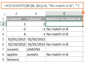
3.1.1 Formula For No Match

=IF(COUNTIF($B:$B, $A2)=0, "No match in B", "")

This formula searches across the entire column B for the value in cell A2. If no match is found, the formula returns “No match in B”, an empty string otherwise.

3.2 Using IF With ISERROR And MATCH

Alternatively, you can use an IF formula with the embedded ISERROR and MATCH functions to achieve the same result.

3.2.1 Formula For No Match

=IF(ISERROR(MATCH($A2,$B$2:$B$10,0)),"No match in B","")

This formula uses the MATCH function to find the position of the value in cell A2 within the range B2:B10. If the value is not found, MATCH returns an error, and ISERROR returns TRUE. The IF formula then returns “No match in B”.

3.3 Using Array Formula

Another way to achieve this is by using an array formula.

3.3.1 Formula For No Match

=IF(SUM(--($B$2:$B$10=$A2))=0, " No match in B", "")

Remember to press Ctrl + Shift + Enter to enter it correctly. This formula checks if the value in cell A2 exists in the range B2:B10. If it does not, the SUM function returns 0, and the IF formula returns “No match in B”.

3.4 Identifying Both Matches And Differences

To identify both matches and differences with a single formula, put some text for matches in the empty double quotes (“”) in any of the above formulas.

3.4.1 Formula For Matches And Differences

=IF(COUNTIF($B:$B, $A2)=0, "No match in B", "Match in B")

This formula returns “No match in B” if the value in A2 is not found in column B, and “Match in B” if it is found.

4. How Can I Compare Two Lists In Excel And Pull Matching Entries?

To compare two lists in Excel and pull matching entries, you can use functions like VLOOKUP, INDEX MATCH, or XLOOKUP.

Answer: When the goal is to not only match two columns but also retrieve corresponding data from the matching entries, Excel offers functions like VLOOKUP, INDEX MATCH, and XLOOKUP. VLOOKUP is straightforward for simple lookups, while INDEX MATCH provides more flexibility, especially when dealing with complex data arrangements. XLOOKUP, available in Excel 2021 and Excel 365, combines the strengths of both and simplifies the lookup process further.

4.1 Using VLOOKUP

The VLOOKUP function is used to search for a value in the first column of a range and return a value in the same row from another column in the range.

4.1.1 Formula For Pulling Matching Entries

=VLOOKUP(D2, $A$2:$B$6, 2, FALSE)

This formula compares the product names in column D against the names in column A and pulls a corresponding sales figure from column B if a match is found. If no match is found, the #N/A error is returned.

4.2 Using INDEX MATCH

The INDEX MATCH combination is a more flexible alternative to VLOOKUP. The MATCH function finds the position of a value in a range, and the INDEX function returns the value at that position in another range.

4.2.1 Formula For Pulling Matching Entries

=INDEX($B$2:$B$6, MATCH($D2, $A$2:$A$6, 0))

4.3 Using XLOOKUP

The XLOOKUP function, available in Excel 2021 and Excel 365, is a more powerful and versatile function that combines the strengths of VLOOKUP and INDEX MATCH.

4.3.1 Formula For Pulling Matching Entries

=XLOOKUP(D2, $A$2:$A$6, $B$2:$B$6)

5. How Do I Compare Two Lists And Highlight Matches And Differences Using Conditional Formatting?

To compare two lists and highlight matches and differences, you can use Excel’s Conditional Formatting feature with formulas.

Answer: Conditional formatting is a powerful feature in Excel for visually highlighting matches and differences between two lists. By using formulas in conditional formatting rules, you can automatically shade cells based on whether their values are unique to one list or present in both. This visual representation makes it easier to quickly identify and analyze the data.

5.1 Highlighting Matches And Differences In Each Row

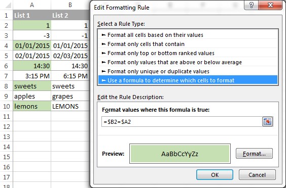
To compare two columns and highlight cells in column A that have identical entries in column B in the same row, use the following steps.

5.1.1 Highlighting Matches

Select the cells you want to highlight.
Click Conditional formatting > New Rule… > Use a formula to determine which cells to format.
Create a rule with the formula:

=$B2=$A2

Assuming that row 2 is the first row with data, not including the column header.

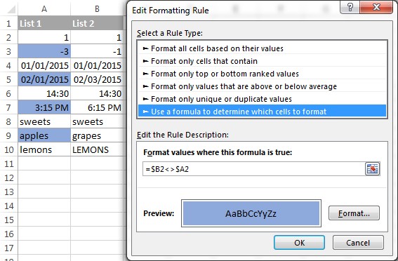
5.1.2 Highlighting Differences

To highlight differences between column A and B, create a rule with this formula:

=$B2<>$A2

5.2 Highlighting Unique Entries In Each List

To highlight the items that are only in one list, follow these steps.

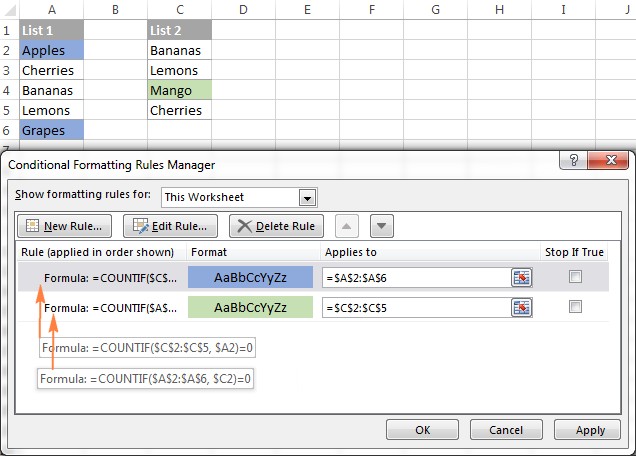
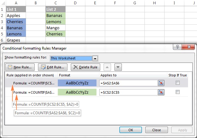
5.2.1 Highlighting Unique Values In List 1 (Column A)

=COUNTIF($C$2:$C$5, $A2)=0

5.2.2 Highlighting Unique Values In List 2 (Column C)

=COUNTIF($A$2:$A$6, $C2)=0

5.3 Highlighting Matches (Duplicates) Between 2 Columns

To highlight the matches between two columns, adjust the COUNTIF formulas so that they find the matches rather than differences.

5.3.1 Highlighting Matches In List 1 (Column A)

=COUNTIF($C$2:$C$5, $A2)>0

5.3.2 Highlighting Matches In List 2 (Column C)

=COUNTIF($A$2:$A$6, $C2)>0

6. How Can I Highlight Row Differences And Matches In Multiple Columns?

When comparing values in several columns row by row, the quickest way to highlight matches is creating a conditional formatting rule, and the fastest way to shade differences is using the Go To Special feature.

Answer: For scenarios involving multiple columns, Excel’s conditional formatting can be used to highlight entire rows based on matching values. Additionally, the “Go To Special” feature offers a quick way to identify and highlight cells with different values within each row. Combining these techniques allows for a comprehensive visual comparison of data across multiple columns.

6.1 Comparing Multiple Columns And Highlighting Row Matches

To highlight rows that have identical values in all columns, create a conditional formatting rule based on one of the following formulas.

6.1.1 Using AND Formula

=AND($A2=$B2, $A2=$C2)

6.1.2 Using COUNTIF Formula

=COUNTIF($A2:$C2, $A2)=3

Where A2, B2, and C2 are the top-most cells and 3 is the number of columns to compare.

6.2 Comparing Multiple Columns And Highlighting Row Differences

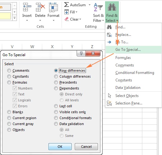
To quickly highlight cells with different values in each individual row, you can use Excel’s Go To Special feature.

6.2.1 Steps To Highlight Row Differences

Select the range of cells you want to compare.
On the Home tab, go to Editing group, and click Find & Select > Go To Special… Then select Row differences and click the OK button.
The cells whose values are different from the comparison cell in each row are colored. If you want to shade the highlighted cells in some color, simply click the Fill Color icon on the ribbon and select the color of your choosing.

7. What Is The Simplest Way To Compare Two Cells In Excel?

Comparing two cells is a straightforward task in Excel, involving the use of basic comparison formulas.

Answer: Comparing two cells in Excel is straightforward using simple IF formulas to check for matches or differences. This method is quick and efficient for direct comparisons.

7.1 Using IF Formula For Matches

To compare cells A1 and C1 for matches, use the following formula:

=IF(A1=C1, "Match", "")

7.2 Using IF Formula For Differences

To compare cells A1 and C1 for differences, use the following formula:

=IF(A1<>C1, "Difference", "")

8. Are There Formula-Free Ways To Compare Two Columns/Lists In Excel?

While formulas are powerful, there are also formula-free ways to compare columns in Excel using tools like the Compare Two Tables add-in.

Answer: For users who prefer not to use formulas, Excel add-ins like “Compare Two Tables” provide a formula-free solution. These tools simplify the comparison process by identifying matches and differences with just a few clicks, making it accessible for users of all skill levels.

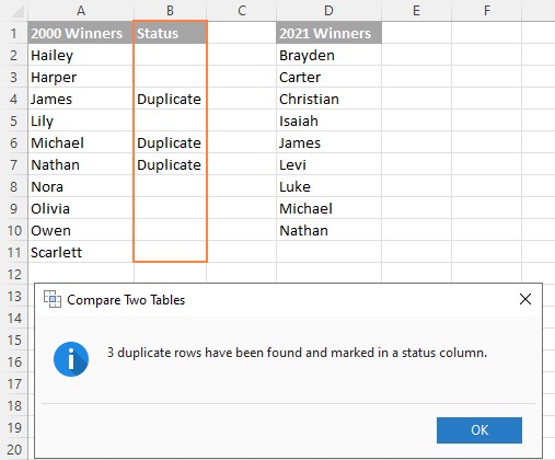
8.1 Using Compare Two Tables Add-In

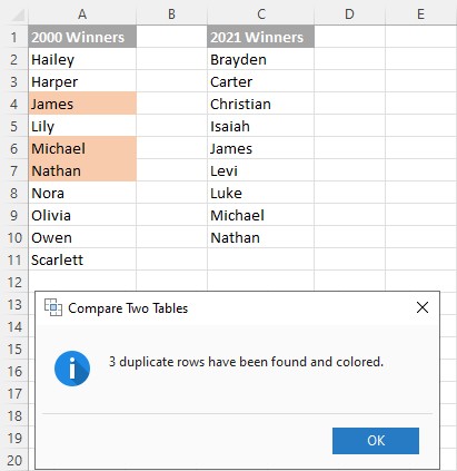
The Compare Two Tables add-in, included in the Ultimate Suite, can compare two tables or lists by any number of columns and both identify matches/differences and highlight them.

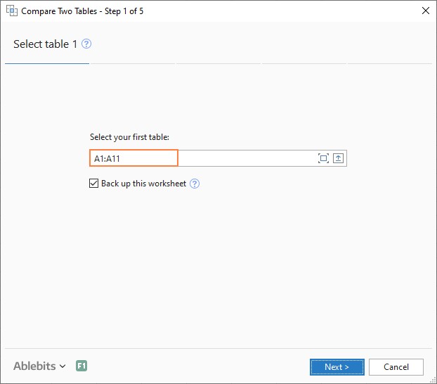
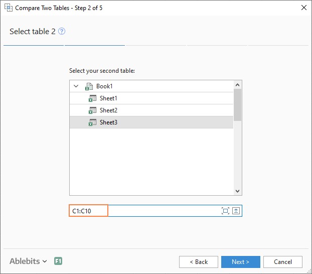
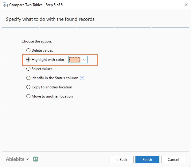
8.1.1 Steps To Compare Two Lists Using Compare Two Tables

Click the Compare Tables button on the Ablebits Data tab.
Select the first column/list and click Next.
Select the second column/list and click Next.
Choose what kind of data to look for:
- Duplicate values (matches) – the items that exist in both lists.
- Unique values (differences) – the items that are present in list 1, but not in list 2.
Select the columns for comparison.
In the final step, you choose how to deal with the found items and click Finish.

9. FAQ About Comparing And Highlighting Differences In Excel

9.1 How do I compare two columns in Excel for exact matches?

Use the EXACT function within an IF formula to perform a case-sensitive comparison. For example: =IF(EXACT(A2, B2), "Match", "").

9.2 Can I compare two columns and return a value from a third column if there’s a match?

Yes, use the VLOOKUP, INDEX MATCH, or XLOOKUP functions. For example: =VLOOKUP(A2, $B$2:$C$10, 2, FALSE) will return the value from column C if A2 matches a value in column B.

9.3 How can I highlight duplicate values in two columns?

Use conditional formatting with the formula =COUNTIF($B:$B, $A2)>0 to highlight values in column A that also appear in column B.

9.4 What is the best way to compare multiple columns for the same value in each row?

Use the AND function within an IF formula or the COUNTIF function. For example: =IF(AND(A2=B2, A2=C2), "Match", "") or =IF(COUNTIF($A2:$C2, $A2)=3, "Match", "").

9.5 How do I find unique values in two columns?

Use the COUNTIF function within an IF formula to check if a value from one column does not exist in the other column. For example: =IF(COUNTIF($B:$B, $A2)=0, "Unique", "").

9.6 How can I highlight an entire row if there is a difference in any of the columns?

Use conditional formatting with a formula that checks for differences across the row. For example: =OR(A2<>B2, A2<>C2) will highlight the row if there are any differences between columns A, B, and C.

9.7 Can I compare two columns for partial matches?

Yes, you can use the SEARCH function within an IF formula. For example: =IF(ISNUMBER(SEARCH(A2, B2)), "Partial Match", "") will check if A2 is a substring of B2.

9.8 What is the difference between VLOOKUP and INDEX MATCH?

VLOOKUP is simpler for basic lookups but requires the lookup value to be in the first column of the range. INDEX MATCH is more flexible and can handle lookups in any column.

9.9 How do I ignore case when comparing two columns?

Use the UPPER or LOWER functions to convert both columns to the same case before comparing. For example: =IF(UPPER(A2)=UPPER(B2), "Match", "").

9.10 Is there a way to compare two Excel files for differences?

Yes, you can use the “Compare Two Tables” add-in or other third-party tools to compare entire Excel files for differences.

10. Conclusion

Comparing and highlighting differences in Excel is essential for data analysis and decision-making. By using the techniques described in this guide, you can easily identify matches and differences, pull matching entries, and highlight important data points. Whether you prefer using formulas or formula-free tools, Excel provides a variety of options to suit your needs.

Ready to make data comparison easier? Visit COMPARE.EDU.VN to find the best comparison guides and make informed decisions. Check out our detailed comparisons and reviews to streamline your decision-making process.

Contact Us:

Address: 333 Comparison Plaza, Choice City, CA 90210, United States
WhatsApp: +1 (626) 555-9090
Website: compare.edu.vn