How To Compare 2 Sheets In Excel For Matches?

Comparing two sheets in Excel for matches is straightforward when you use the right techniques, and compare.edu.vn provides a comprehensive guide to help you through the process. By using functions like MATCH and conditional formatting, you can easily identify matching data, highlight differences, and streamline your data analysis; explore more on data comparison, spreadsheet analysis and Excel tutorials for in-depth understanding.

1. What Is The Best Way To Compare Two Sheets In Excel For Matches?

The best way to compare two sheets in Excel for matches is to use a combination of Excel functions such as MATCH, VLOOKUP, and conditional formatting. These tools allow you to quickly identify identical entries, highlight differences, and ensure data consistency across your spreadsheets. Let’s explore these methods in detail.

1.1 Using The MATCH Function

The MATCH function is a powerful tool for finding the position of a specific value in a range of cells. It’s particularly useful for comparing two sheets to see if a value from one sheet exists in another.

How it works:

• The MATCH function searches for a specified item in a range of cells and returns the position of that item within the range.
• If the value is found, MATCH returns a number representing its position.
• If the value is not found, MATCH returns an error (#N/A).

Step-by-step guide:

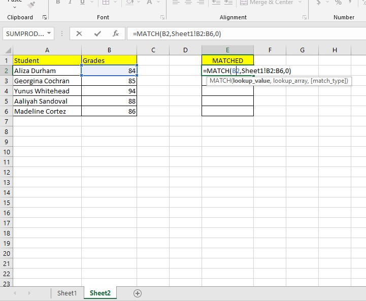
1. Prepare Your Worksheets: Ensure both worksheets you want to compare are open in the same Excel workbook.

2. Select a Helper Column: In the sheet where you want to identify matches, select an empty column next to the data you want to check.

3. Enter the MATCH Formula: In the first cell of the helper column, enter the following formula:

   =MATCH(A2,Sheet2!A:A,0)

   • A2 is the cell in the current sheet that you want to find in the other sheet.
   • Sheet2!A:A is the range of cells in Sheet2 where you’re looking for the value.
   • 0 specifies an exact match.

4. Apply the Formula to the Entire Column: Drag the fill handle (the small square at the bottom-right of the cell) down to apply the formula to all relevant rows.

5. Interpret the Results:

   • A number indicates the position of the matched value in Sheet2.
   • #N/A means the value from Sheet1 was not found in Sheet2.

Example:

Suppose you have a list of customer IDs in Sheet1, column A, starting from A2. You want to check if these IDs exist in Sheet2, column A. In Sheet1, in cell B2, you would enter:

=MATCH(A2,Sheet2!A:A,0)

Drag this formula down column B. If MATCH returns a number, the customer ID exists in Sheet2. If it returns #N/A, the ID is not present in Sheet2.

1.2 Using The VLOOKUP Function

The VLOOKUP function is another excellent tool for comparing data across two sheets. It searches for a value in the first column of a range and returns a value in the same row from a column you specify.

How it works:

• VLOOKUP looks for a specified value in the leftmost column of a table range.
• Once it finds a match, it returns a value from a column in the same row, based on the column index number you provide.
• If no match is found, VLOOKUP returns an error (#N/A).

Step-by-step guide:

1. Prepare Your Worksheets: Ensure both sheets are in the same Excel workbook.

2. Select a Helper Column: In the sheet where you want to display the results, select an empty column next to your data.

3. Enter the VLOOKUP Formula: In the first cell of the helper column, enter the following formula:

   =VLOOKUP(A2,Sheet2!A:B,2,FALSE)

   • A2 is the cell in the current sheet containing the value you want to find in Sheet2.
   • Sheet2!A:B is the range in Sheet2 where you want to search for the value and retrieve related data. Adjust the range if your data spans more columns.
   • 2 is the column index number in Sheet2 from which to return a value. In this example, it’s the second column.
   • FALSE specifies an exact match.

4. Apply the Formula to the Entire Column: Drag the fill handle down to apply the formula to all relevant rows.

5. Interpret the Results:

   • If VLOOKUP returns a value, it means the lookup value was found, and the corresponding value from the specified column is displayed.
   • #N/A means the value was not found in Sheet2.

Example:

Imagine you have a list of product codes in Sheet1, column A, starting from A2, and you want to retrieve the corresponding product names from Sheet2, where product codes are in column A and product names are in column B. In Sheet1, in cell B2, you would enter:

=VLOOKUP(A2,Sheet2!A:B,2,FALSE)

Drag this formula down column B. If VLOOKUP returns a product name, the code exists in Sheet2, and you see the corresponding name. If it returns #N/A, the product code is not in Sheet2.

1.3 Using Conditional Formatting

Conditional formatting is a powerful feature that allows you to highlight cells based on specific criteria. This is particularly useful for visually identifying matches or differences between two sheets.

How it works:

• Conditional formatting applies formatting (e.g., cell color, font style) to cells that meet certain conditions.
• You can set up rules to highlight cells in one sheet that have matching values in another sheet.

Step-by-step guide:

1. Select the Range: In the first sheet, select the range of cells you want to compare.

2. Open Conditional Formatting: Go to the “Home” tab, click on “Conditional Formatting,” and select “New Rule.”

3. Create a New Rule: Choose “Use a formula to determine which cells to format.”

4. Enter the Formula: Enter a formula that checks for matches in the other sheet. For example:

   =ISNUMBER(MATCH(A1,Sheet2!A:A,0))

   • A1 is the first cell in your selected range.
   • Sheet2!A:A is the range in Sheet2 where you are looking for matches.

5. Set the Formatting: Click “Format” and choose the formatting style you want to apply to the matching cells (e.g., fill color, font color).

6. Apply the Rule: Click “OK” to apply the rule. Excel will now highlight all cells in the selected range that have a match in Sheet2.

Example:

Suppose you have a list of email addresses in Sheet1, column A, and you want to highlight those addresses that also appear in Sheet2, column A.

1. Select the range A1:A100 in Sheet1.
2. Go to “Home” > “Conditional Formatting” > “New Rule.”
3. Choose “Use a formula to determine which cells to format.”
4. Enter the formula: =ISNUMBER(MATCH(A1,Sheet2!A:A,0))
5. Click “Format,” choose a fill color (e.g., green), and click “OK.”
6. Click “OK” to apply the rule.

Now, all email addresses in Sheet1 that also exist in Sheet2 will be highlighted in green.

1.4 Combining Methods for Comprehensive Comparison

For a thorough comparison, it’s often beneficial to combine these methods. For instance, you can use MATCH or VLOOKUP to identify matches and then use conditional formatting to highlight these matches for a visual overview.

1.5 Other Excel Functions for Comparison

Besides MATCH and VLOOKUP, other Excel functions can aid in comparing sheets:

• EXACT Function: Compares two text strings and returns TRUE if they are exactly the same, including case.
• IF Function: Performs a logical test and returns one value if the condition is TRUE and another value if it is FALSE.

Example using EXACT and IF:

=IF(EXACT(Sheet1!A1,Sheet2!A1),"Match","No Match")

This formula compares the values in cell A1 of Sheet1 and Sheet2. If they are exactly the same, it returns “Match”; otherwise, it returns “No Match.”

2. What Are The Steps To Highlight Matched Data From A Separate Worksheet In Excel?

Highlighting matched data from a separate worksheet in Excel involves using conditional formatting with a formula that checks for matches in the other sheet. Here’s a detailed guide on how to accomplish this.

2.1 Step-By-Step Guide To Highlight Matched Data

1. Select the Data Range: In the worksheet where you want to highlight the matched data, select the range of cells you want to format. For example, if you want to compare the data in column A, select the entire column or the specific range you are interested in (e.g., A1:A100).

2. Open Conditional Formatting:

   • Go to the “Home” tab on the Excel ribbon.
   • Click on “Conditional Formatting” in the “Styles” group.
   • Select “New Rule…” from the dropdown menu.

3. Choose the Rule Type: In the “New Formatting Rule” dialog box, select “Use a formula to determine which cells to format.” This option allows you to use a formula to define the condition for formatting.

4. Enter the Formula: In the formula box, enter a formula that checks for matches in the other worksheet. The MATCH function is commonly used for this purpose because it returns the position of a value in a range, or an error if the value is not found. Here’s an example formula:

   =ISNUMBER(MATCH(A1,Sheet2!$A$1:$A$100,0))

   • A1 is the first cell in the selected range of your current worksheet. Excel will adjust this reference for each cell in the range.
   • Sheet2!$A$1:$A$100 is the range of cells in the second worksheet that you want to compare against. The $ signs make the cell references absolute, so they don’t change when the conditional formatting is applied to other cells.
   • 0 specifies that the MATCH function should find an exact match.
   • ISNUMBER checks whether the result of the MATCH function is a number (i.e., a match was found). If a match is found, MATCH returns a number, and ISNUMBER returns TRUE; otherwise, MATCH returns an error, and ISNUMBER returns FALSE.

5. Set the Formatting:

   • Click the “Format…” button in the “New Formatting Rule” dialog box to specify how you want the matched cells to be highlighted.
   • In the “Format Cells” dialog box, you can choose various formatting options, such as:
     • Font: Change the font type, style, size, and color.
     • Border: Add or modify cell borders.
     • Fill: Change the background color of the cell. Choose a color that will make the matched cells stand out (e.g., green, yellow, or light blue).
   • After selecting your desired formatting options, click “OK” to close the “Format Cells” dialog box.

6. Apply the Rule:

   • Back in the “New Formatting Rule” dialog box, you’ll see a preview of the formatting you’ve selected.
   • Click “OK” to apply the conditional formatting rule to your selected range.

7. Review the Results: Excel will now highlight all cells in your selected range that have a matching value in the specified range of the second worksheet.

2.2 Example Scenario

Let’s say you have two worksheets: “CustomerList” and “Orders.” In “CustomerList,” column A contains a list of customer IDs, and in “Orders,” column B also contains customer IDs. You want to highlight the customer IDs in “CustomerList” that appear in “Orders.”

1. Select the Range: In the “CustomerList” worksheet, select the range A1:A100 (assuming you have 100 customer IDs).

2. Open Conditional Formatting: Go to “Home” > “Conditional Formatting” > “New Rule…”

3. Choose the Rule Type: Select “Use a formula to determine which cells to format.”

4. Enter the Formula: Enter the following formula:

   =ISNUMBER(MATCH(A1,Orders!$B$1:$B$100,0))

5. Set the Formatting: Click “Format…”, choose a fill color (e.g., green), and click “OK.”

6. Apply the Rule: Click “OK” to apply the conditional formatting rule.

Now, all customer IDs in the “CustomerList” worksheet that also appear in the “Orders” worksheet will be highlighted in green.

2.3 Additional Tips

• Adjust Cell References: Make sure to adjust the cell references in the formula to match the actual location of your data.
• Absolute vs. Relative References: Use absolute references ($) to prevent the row and column references from changing when the conditional formatting is applied to other cells. Use relative references when you want the references to adjust based on the cell’s position.
• Manage Rules: You can manage and edit conditional formatting rules by going to “Home” > “Conditional Formatting” > “Manage Rules…” This allows you to edit, delete, or change the order of your rules.

3. What Formula Can I Use For Matching Values In Microsoft Excel?

Several formulas can be used for matching values in Microsoft Excel, depending on the specific requirements. The most common and effective formulas include MATCH, VLOOKUP, INDEX & MATCH, and COUNTIF. Each of these formulas has its strengths and is suitable for different scenarios.

3.1 The MATCH Formula

The MATCH formula is used to find the position of a specified value within a range of cells. It returns the relative position of the item in the array.

Syntax:

=MATCH(lookup_value, lookup_array, [match_type])

• lookup_value: The value you want to find.
• lookup_array: The range of cells being searched.
• match_type: (Optional) Specifies how Excel matches the lookup_value in the lookup_array. Common values are:
  • 0: Exact match (most commonly used for matching values).
  • 1: Finds the largest value that is less than or equal to the lookup_value (requires the lookup_array to be sorted in ascending order).
  • -1: Finds the smallest value that is greater than or equal to the lookup_value (requires the lookup_array to be sorted in descending order).

Example:

Suppose you have a list of product names in cells A1:A10, and you want to find the position of “Product C.” The formula would be:

=MATCH("Product C", A1:A10, 0)

If “Product C” is in cell A5, the formula will return 5. If “Product C” is not found, the formula will return #N/A.

Use Cases:

• Finding the position of an item in a list.
• Validating data entries.
• Combining with other functions like INDEX for more complex lookups.

3.2 The VLOOKUP Formula

The VLOOKUP (Vertical Lookup) formula is used to find a value in the first column of a table and return a value in the same row from a column you specify.

Syntax:

=VLOOKUP(lookup_value, table_array, col_index_num, [range_lookup])

• lookup_value: The value you want to find.
• table_array: The range of cells that makes up the table where you want to look for the value.
• col_index_num: The column number in the table_array from which the matching value must be returned.
• range_lookup: (Optional) Specifies whether to find an exact or approximate match:
  • TRUE or omitted: Approximate match (requires the first column of the table_array to be sorted in ascending order).
  • FALSE: Exact match (most commonly used for matching values).

Example:

Suppose you have a table with product codes in column A (A1:A10) and corresponding product names in column B (B1:B10). You want to find the name of the product with code “123.” The formula would be:

=VLOOKUP("123", A1:B10, 2, FALSE)

If the product code “123” is in cell A4, and the corresponding product name is “Product D” in cell B4, the formula will return “Product D.” If “123” is not found, the formula will return #N/A.

Use Cases:

• Retrieving data from a table based on a unique identifier.
• Looking up prices, names, or other related information.
• Useful when the lookup value is in the first column of the table.

3.3 The INDEX & MATCH Combination

The INDEX and MATCH combination is a more flexible alternative to VLOOKUP. It can look up values in any column of a table, and it is not limited to looking up values in the first column.

Syntax:

• INDEX:

  =INDEX(array, row_num, [column_num])

• MATCH:

  =MATCH(lookup_value, lookup_array, [match_type])

Combined Formula:

=INDEX(return_array, MATCH(lookup_value, lookup_array, 0))

• return_array: The range of cells from which to return a value.
• lookup_value: The value you want to find.
• lookup_array: The range of cells being searched.

Example:

Suppose you have product codes in column A (A1:A10) and product names in column B (B1:B10). You want to find the name of the product with code “123.” The formula would be:

=INDEX(B1:B10, MATCH("123", A1:A10, 0))

If the product code “123” is in cell A4, and the corresponding product name is “Product D” in cell B4, the formula will return “Product D.” If “123” is not found, the formula will return #N/A.

Use Cases:

• More flexible than VLOOKUP because it can look up values in any column.
• Can handle more complex lookups and data retrieval scenarios.
• Useful when the table structure might change, and you don’t want to rely on column numbers.

3.4 The COUNTIF Formula

The COUNTIF formula is used to count the number of cells within a range that meet a given criterion. It can be used to check if a value exists in a list.

Syntax:

=COUNTIF(range, criteria)

• range: The range of cells you want to evaluate.
• criteria: The condition that determines which cells will be counted.

Example:

Suppose you have a list of customer IDs in cells A1:A10, and you want to check if the customer ID “456” exists in the list. The formula would be:

=COUNTIF(A1:A10, "456")

If “456” is in the list, the formula will return 1 (or more, if it appears multiple times). If “456” is not found, the formula will return 0.

Use Cases:

• Checking if a value exists in a list.
• Counting the number of times a value appears in a range.
• Validating data entries.

3.5 Choosing The Right Formula

The choice of formula depends on your specific needs:

• Use MATCH when you need to find the position of a value in a list.
• Use VLOOKUP when you need to retrieve data from a table based on a unique identifier, and the lookup value is in the first column of the table.
• Use INDEX & MATCH for more flexible lookups that are not limited to the first column of a table.
• Use COUNTIF when you need to check if a value exists in a list or count the number of times it appears.

4. Can I Use Index Match In Different Sheets?

Yes, you can absolutely use the INDEX MATCH combination in different sheets within the same Excel workbook. This is one of the strengths of INDEX MATCH compared to VLOOKUP, as it provides more flexibility in looking up values across multiple sheets.

4.1 Syntax For INDEX MATCH Across Different Sheets

When using INDEX MATCH across different sheets, you need to specify the sheet name in the formula for both the INDEX and MATCH functions.

Syntax:

=INDEX(Sheet2!return_array, MATCH(Sheet1!lookup_value, Sheet2!lookup_array, 0))

• Sheet2!return_array: The range of cells from which to return a value, located in Sheet2.
• Sheet1!lookup_value: The value you want to find, located in Sheet1.
• Sheet2!lookup_array: The range of cells being searched, located in Sheet2.

4.2 Step-By-Step Example

Let’s illustrate with an example. Suppose you have two sheets: “Products” and “Prices.”

• Products Sheet: Contains a list of product codes in column A (A1:A10) and corresponding product names in column B (B1:B10).
• Prices Sheet: Contains the same product codes in column A (A1:A10) and corresponding prices in column C (C1:C10).

You want to find the price of a product given its name, with the name located in the “Products” sheet and the price in the “Prices” sheet.

Steps:

1. Select the Cell for the Result: In the “Products” sheet, select the cell where you want the price to appear (e.g., C1).

2. Enter the INDEX MATCH Formula: In cell C1 of the “Products” sheet, enter the following formula:

   =INDEX(Prices!C1:C10, MATCH(B1, Prices!A1:A10, 0))

   • Prices!C1:C10: This is the range of cells containing the prices you want to retrieve, located in the “Prices” sheet.
   • B1: This is the cell in the “Products” sheet containing the product name you want to look up.
   • Prices!A1:A10: This is the range of cells in the “Prices” sheet containing the product codes.

3. Apply the Formula: Press Enter to apply the formula. The price of the product corresponding to the name in B1 will appear in C1.

4. Drag the Formula Down: Drag the fill handle (the small square at the bottom-right of the cell) down to apply the formula to all relevant rows.

Now, for each product name in column B of the “Products” sheet, the corresponding price from the “Prices” sheet will be displayed in column C.

4.3 Advantages Of Using INDEX MATCH Across Sheets

• Flexibility: INDEX MATCH is more flexible than VLOOKUP because it can look up values in any column, not just the first one.
• Efficiency: It is more efficient because it only looks at the necessary columns, rather than the entire table.
• Robustness: It is more robust because it does not rely on column numbers, which can change if columns are inserted or deleted.

4.4 Practical Tips

• Use Absolute References: To prevent the cell references from changing when you drag the formula down, use absolute references ($). For example:

  =INDEX(Prices!$C$1:$C$10, MATCH(B1, Prices!$A$1:$A$10, 0))

• Error Handling: If a match is not found, the formula will return #N/A. You can use the IFERROR function to handle this error and display a more user-friendly message. For example:

  =IFERROR(INDEX(Prices!$C$1:$C$10, MATCH(B1, Prices!$A$1:$A$10, 0)), "Not Found")

• Consistent Data: Ensure that the lookup values in both sheets are consistent in terms of formatting and data type.

4.5 Example Scenario

Imagine you are managing inventory for a retail business. You have two sheets:

• Inventory: Contains a list of product IDs in column A and product descriptions in column B.
• Sales: Contains a list of product IDs in column A and quantities sold in column C.

You want to add the product description to the “Sales” sheet based on the product ID.

1. Select the Cell: In the “Sales” sheet, select the cell where you want the product description to appear (e.g., B1).

2. Enter the Formula: Enter the following formula in cell B1:

   =INDEX(Inventory!$B$1:$B$100, MATCH(A1, Inventory!$A$1:$A$100, 0))

3. Apply the Formula: Press Enter and drag the formula down to apply it to all relevant rows.

Now, the “Sales” sheet will display the product description for each product ID, pulled from the “Inventory” sheet.

5. Can I Use The VLOOKUP Formula To Compare Two Sheets?

Yes, you can use the VLOOKUP formula to compare two sheets in Excel. VLOOKUP is primarily designed to search for a value in the first column of a table and return a value from another column in the same row. When comparing two sheets, you can use VLOOKUP to check if values from one sheet exist in another and retrieve corresponding data if a match is found.

5.1 How To Use VLOOKUP To Compare Two Sheets

Here’s a step-by-step guide on how to use VLOOKUP to compare data in two different sheets:

1. Prepare Your Worksheets:

   • Ensure both worksheets are in the same Excel workbook.
   • Identify the common column (the column with the same type of data) that you will use for comparison. This column must be the first column in the table_array argument of the VLOOKUP function.

2. Select the Worksheet for Results:

   • Choose the worksheet where you want to display the results of the comparison. This is typically the sheet where you want to add information about whether a match was found.

3. Enter the VLOOKUP Formula:

   • In the chosen worksheet, select the cell where you want the result to appear.
   • Enter the VLOOKUP formula with the appropriate arguments:

   =VLOOKUP(lookup_value, table_array, col_index_num, [range_lookup])

   • lookup_value: This is the value you want to find in the other sheet. It is usually a cell reference in the current sheet.
   • table_array: This is the range of cells in the other sheet where you want to search for the lookup_value. Make sure the common column is the first column in this range.
   • col_index_num: This is the column number in the table_array from which to return a value if a match is found. If you only want to check if a match exists, you can use any column number within the range.
   • [range_lookup]: This is an optional argument. Use FALSE for an exact match.

5.2 Example Scenario

Let’s consider a scenario where you have two sheets: “Employees” and “Departments.”

• Employees Sheet: Contains a list of employee IDs in column A and employee names in column B.
• Departments Sheet: Contains employee IDs in column A and department names in column C.

You want to check in the “Employees” sheet which employees are listed in the “Departments” sheet and retrieve their department names.

Steps:

1. Select the Cell for the Result: In the “Employees” sheet, select the cell where you want the department name to appear (e.g., C1).

2. Enter the VLOOKUP Formula: In cell C1 of the “Employees” sheet, enter the following formula:

   =VLOOKUP(A1, Departments!A:C, 3, FALSE)

   • A1: This is the employee ID in the “Employees” sheet that you want to look up in the “Departments” sheet.
   • Departments!A:C: This is the range of cells in the “Departments” sheet where you want to search for the employee ID and retrieve the department name. Column A contains the employee IDs, and column C contains the department names.
   • 3: This specifies that you want to return the value from the third column of the table_array (i.e., the department name).
   • FALSE: This ensures that VLOOKUP looks for an exact match of the employee ID.

3. Apply the Formula: Press Enter to apply the formula. The department name for the employee ID in A1 will appear in C1.

4. Drag the Formula Down: Drag the fill handle down to apply the formula to all relevant rows.

For each employee ID in column A of the “Employees” sheet, the corresponding department name from the “Departments” sheet will be displayed in column C. If an employee ID is not found in the “Departments” sheet, the formula will return #N/A.

5.3 Handling #N/A Errors

When using VLOOKUP, you may encounter #N/A errors if the lookup_value is not found in the table_array. To handle these errors, you can use the IFERROR function.

Syntax:

=IFERROR(VLOOKUP(lookup_value, table_array, col_index_num, [range_lookup]), value_if_error)

• VLOOKUP(lookup_value, table_array, col_index_num, [range_lookup]): This is the VLOOKUP formula as described above.
• value_if_error: This is the value you want to display if the VLOOKUP formula returns an error. It can be a text string (e.g., “Not Found”), a number, or another formula.

Example:

Using the same scenario as above, you can modify the formula in the “Employees” sheet to handle #N/A errors:

=IFERROR(VLOOKUP(A1, Departments!A:C, 3, FALSE), "Not Assigned")

Now, if an employee ID is not found in the “Departments” sheet, the formula will display “Not Assigned” instead of #N/A.

5.4 Conditional Formatting With VLOOKUP

You can also use VLOOKUP in combination with conditional formatting to highlight matches or differences between the two sheets.

Steps:

1. Select the Range: In the worksheet where you want to highlight the matched data, select the range of cells you want to format (e.g., A1:A100 in the “Employees” sheet).

2. Open Conditional Formatting: Go to “Home” > “Conditional Formatting” > “New Rule…”

3. Choose the Rule Type: Select “Use a formula to determine which cells to format.”

4. Enter the Formula: Enter a formula that uses VLOOKUP to check for matches in the other sheet. For example:

   =NOT(ISERROR(VLOOKUP(A1, Departments!A:A, 1, FALSE)))

   • VLOOKUP(A1, Departments!A:A, 1, FALSE): This part of the formula tries to find the employee ID in the “Departments” sheet.
   • ISERROR(...): This checks if the VLOOKUP formula returns an error (i.e., no match is found).
   • NOT(...): This reverses the result, so it returns TRUE if a match is found and FALSE if no match is found.

5. Set the Formatting: Click “Format…”, choose a fill color (e.g., green), and click “OK.”

6. Apply the Rule: Click “OK” to apply the conditional formatting rule.

Now, all employee IDs in the “Employees” sheet that also exist in the “Departments” sheet will be highlighted in green.

6. Frequently Asked Questions (FAQ) On How To Compare Two Excel Sheets For Matching Data

Here are some frequently asked questions (FAQ) on how to compare two Excel sheets for matching data, addressing common issues and providing practical solutions.

6.1 Can I Compare Two Excel Sheets Without Using Formulas?

While formulas provide the most flexible and dynamic way to compare two Excel sheets, you can also use Excel’s built-in features like “Conditional Formatting” and “Remove Duplicates” for basic comparisons without writing formulas.

• Conditional Formatting: Highlight duplicate or unique values directly.
• Remove Duplicates: Quickly identify and remove duplicate rows based on selected columns.

6.2 How Do I Compare Two Excel Sheets With Different Column Orders?

When comparing two sheets with different column orders, you can use the INDEX and MATCH functions in combination. The MATCH function helps find the column position of a specific header in one sheet, and the INDEX function retrieves the value