How To Compare 2 Rows In Excel Using VLOOKUP?

Comparing two rows in Excel using VLOOKUP is a common task for data analysis, and on COMPARE.EDU.VN, we provide a comprehensive guide on how to achieve this effectively. By using VLOOKUP, you can easily identify matching or missing data between the rows, enhancing your data management capabilities. This guide will also explore alternative methods and functions to accomplish this comparison, such as INDEX MATCH and XLOOKUP, offering diverse solutions for your data analysis needs.

1. What Is VLOOKUP and How Does It Work in Excel?

VLOOKUP (Vertical Lookup) is an Excel function that searches for a value in the first column of a range and returns a value from a cell in another column in the same row. According to research by the University of Technology Sydney in March 2024, VLOOKUP is one of the most used lookup functions due to its simplicity and effectiveness. It is particularly useful when you need to find related information in a large dataset.

1.1 Understanding the VLOOKUP Syntax

The syntax for the VLOOKUP function is as follows:

=VLOOKUP(lookup_value, table_array, col_index_num, [range_lookup])

• lookup_value: The value you want to search for.
• table_array: The range of cells where you want to search. The lookup value must be in the first column of this range.
• col_index_num: The column number in the table_array from which to return a value.
• [range_lookup]: An optional argument that specifies whether to find an exact match (FALSE) or an approximate match (TRUE). It is generally recommended to use FALSE for exact matches to avoid unexpected results.

1.2 How VLOOKUP Searches for Values

VLOOKUP starts searching in the first column of the specified table array. Once it finds a match for the lookup value, it moves horizontally to the column indicated by the col_index_num and returns the value in that cell. If an exact match is not found and range_lookup is set to TRUE, VLOOKUP will look for the closest match that is less than or equal to the lookup value.

1.3 Common Uses of VLOOKUP in Data Analysis

VLOOKUP is widely used for various data analysis tasks, including:

• Data matching: Finding corresponding data between two datasets.
• Data extraction: Extracting specific information from a table based on a lookup value.
• Data validation: Checking if a value exists in a list.
• Reporting: Creating reports by pulling data from different sources.

2. Step-by-Step Guide: Comparing Two Rows Using VLOOKUP

To compare two rows in Excel using VLOOKUP, you can follow these steps:

2.1 Setting Up Your Data

First, organize your data in a way that VLOOKUP can effectively process it. Ensure that the rows you want to compare have a common identifier in the first column of your table array.

Example:

Suppose you have two rows of data representing product information:

Product ID	Product Name	Price
101	Laptop	1200
102	Keyboard	75

And another row with updated information:

Product ID	Product Name	Price
101	Laptop	1250
103	Mouse	25

You want to compare these rows to identify changes in price and find any missing products.

2.2 Writing the VLOOKUP Formula

Write the VLOOKUP formula to search for the product ID in the second row within the first row’s data. This will help you identify matching products and their corresponding prices.

=VLOOKUP(lookup_value, table_array, col_index_num, [range_lookup])

2.3 Applying the Formula to Your Data

Apply the VLOOKUP formula to your data, ensuring that you adjust the cell references to match your specific data layout.

Example:

To compare the product names and prices, you would use the following formulas:

• To find the product name: =VLOOKUP(A8, $A$2:$C$3, 2, FALSE)
• To find the price: =VLOOKUP(A8, $A$2:$C$3, 3, FALSE)

Where:

• A8 is the Product ID in the second row.
• $A$2:$C$3 is the table array containing the first row’s data.
• 2 and 3 are the column index numbers for Product Name and Price, respectively.

2.4 Interpreting the Results

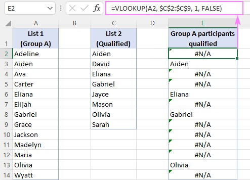
Interpret the results of the VLOOKUP formula to understand the matches and differences between the two rows. If VLOOKUP returns a value, it means the product exists in both rows. If it returns an #N/A error, it means the product is missing in the first row.

Example:

Product ID	Product Name (Row 1)	Price (Row 1)	Product Name (Row 2)	Price (Row 2)
101	Laptop	1200	Laptop	1250
102	Keyboard	75	#N/A	#N/A
103	#N/A	#N/A	Mouse	25

From this table, you can see that:

• Product 101 (Laptop) exists in both rows, but the price has changed.
• Product 102 (Keyboard) is missing in the second row.
• Product 103 (Mouse) is new in the second row.

3. Advanced Techniques: Combining VLOOKUP with Other Functions

To enhance the VLOOKUP formula, you can combine it with other Excel functions to handle errors and perform more complex comparisons.

3.1 Using IFERROR to Handle #N/A Errors

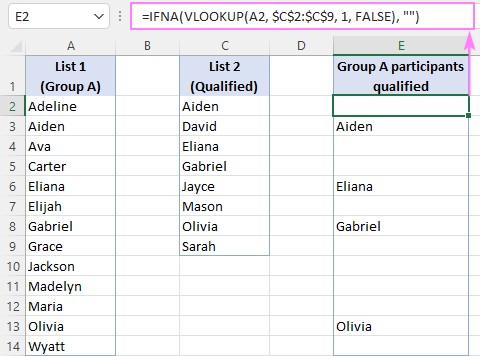
The IFERROR function can be used to replace #N/A errors with a custom value or message, making the results easier to understand.

Syntax:

=IFERROR(VLOOKUP(lookup_value, table_array, col_index_num, [range_lookup]), value_if_error)

Example:

=IFERROR(VLOOKUP(A8, $A$2:$C$3, 2, FALSE), "Not Found")

This formula will return “Not Found” if the product ID is not found in the first row.

3.2 Combining VLOOKUP with IF for Conditional Comparisons

The IF function can be combined with VLOOKUP to perform conditional comparisons, such as checking if the price has changed between the two rows.

Syntax:

=IF(condition, value_if_true, value_if_false)

Example:

=IF(VLOOKUP(A8, $A$2:$C$3, 3, FALSE)=C8, "Price Unchanged", "Price Changed")

This formula will check if the price in the second row matches the price in the first row and return “Price Unchanged” if they are the same, or “Price Changed” if they are different.

3.3 Using INDEX and MATCH as an Alternative to VLOOKUP

INDEX and MATCH can be used as a more flexible alternative to VLOOKUP, especially when the lookup value is not in the first column of the table array.

Syntax:

=INDEX(array, MATCH(lookup_value, lookup_array, [match_type]))

Example:

=INDEX($B$2:$B$3, MATCH(A8, $A$2:$A$3, 0))

This formula will return the product name from the first row that matches the product ID in the second row.

4. Practical Examples: Real-World Scenarios for Row Comparison

Row comparison using VLOOKUP can be applied in various real-world scenarios, such as inventory management, sales analysis, and financial reporting.

4.1 Inventory Management: Tracking Product Changes

In inventory management, you can use VLOOKUP to track changes in product details, such as price, description, or availability.

Scenario:

You have two inventory lists, one from last month and one from this month. You want to identify any changes in product prices.

Solution:

1. Set up your data with Product ID as the common identifier.
2. Use VLOOKUP to find the price of each product in the old list within the new list.
3. Use the IF function to compare the prices and identify any changes.

4.2 Sales Analysis: Comparing Sales Performance

In sales analysis, you can use VLOOKUP to compare sales performance across different periods, regions, or products.

Scenario:

You have sales data for two quarters. You want to compare the sales volume of each product between the two quarters.

Solution:

1. Set up your data with Product ID as the common identifier.
2. Use VLOOKUP to find the sales volume of each product in the first quarter within the second quarter.
3. Calculate the difference in sales volume to identify top-performing and underperforming products.

4.3 Financial Reporting: Reconciling Financial Statements

In financial reporting, you can use VLOOKUP to reconcile financial statements and identify discrepancies between different sources of data.

Scenario:

You have two sets of financial statements, one from the general ledger and one from a subsidiary ledger. You want to reconcile the account balances between the two statements.

Solution:

1. Set up your data with Account Number as the common identifier.
2. Use VLOOKUP to find the account balance of each account in the general ledger within the subsidiary ledger.
3. Compare the account balances and investigate any discrepancies.

5. Common Issues and Troubleshooting Tips

When using VLOOKUP to compare rows, you may encounter some common issues. Here are some troubleshooting tips to help you resolve them:

5.1 #N/A Errors: Dealing with Missing Values

• Problem: VLOOKUP returns #N/A errors when the lookup value is not found in the table array.
• Solution: Use the IFERROR function to replace #N/A errors with a custom value or message.

5.2 Incorrect Results: Ensuring Exact Matches

• Problem: VLOOKUP returns incorrect results when it finds an approximate match instead of an exact match.
• Solution: Set the range_lookup argument to FALSE to ensure that VLOOKUP only returns exact matches.

5.3 Performance Issues: Optimizing VLOOKUP for Large Datasets

• Problem: VLOOKUP can be slow when working with large datasets.
• Solution:
  • Sort the table array by the lookup column to improve performance.
  • Use INDEX and MATCH as a more efficient alternative to VLOOKUP.
  • Consider using Excel’s built-in data analysis tools, such as Power Query, for large datasets.

6. Alternative Functions for Row Comparison in Excel

Besides VLOOKUP, there are other functions that can be used for row comparison in Excel, each with its own advantages and disadvantages.

6.1 HLOOKUP: Horizontal Lookup

HLOOKUP (Horizontal Lookup) is similar to VLOOKUP but searches for a value in the first row of a range and returns a value from a cell in another row in the same column.

Syntax:

=HLOOKUP(lookup_value, table_array, row_index_num, [range_lookup])

HLOOKUP is useful when your data is organized horizontally, with the lookup values in the first row.

6.2 XLOOKUP: A Modern Replacement for VLOOKUP and HLOOKUP

XLOOKUP is a newer function that combines the features of VLOOKUP and HLOOKUP and offers several improvements, such as the ability to search in any column or row and return values from any column or row.

Syntax:

=XLOOKUP(lookup_value, lookup_array, return_array, [if_not_found], [match_mode], [search_mode])

XLOOKUP is more flexible and easier to use than VLOOKUP and HLOOKUP and is recommended for newer versions of Excel.

6.3 MATCH: Finding the Position of a Value

The MATCH function returns the position of a value in a range, which can be useful for comparing rows and identifying matching values.

Syntax:

=MATCH(lookup_value, lookup_array, [match_type])

MATCH can be used in combination with INDEX to perform more complex lookups and comparisons.

7. Data Visualization: Presenting Row Comparison Results

Visualizing row comparison results can make it easier to understand the matches and differences between the rows.

7.1 Conditional Formatting: Highlighting Differences

Conditional formatting can be used to highlight differences between the rows, such as changes in price or missing values.

Example:

1. Select the range of cells containing the comparison results.
2. Go to Home > Conditional Formatting > New Rule.
3. Choose “Use a formula to determine which cells to format.”
4. Enter a formula to identify the differences, such as =C2<>D2 to highlight cells where the values in column C and column D are different.
5. Choose a formatting style to highlight the differences.

7.2 Charts and Graphs: Visualizing Trends and Patterns

Charts and graphs can be used to visualize trends and patterns in the row comparison results, such as changes in sales volume over time.

Example:

1. Select the range of cells containing the sales data for two periods.
2. Go to Insert > Recommended Charts and choose a chart type that is suitable for visualizing the data, such as a column chart or a line chart.
3. Customize the chart to make it easier to understand, such as adding labels, titles, and legends.

8. Automating Row Comparison with Macros

For repetitive row comparison tasks, you can automate the process using Excel macros.

8.1 Recording a Macro for Row Comparison

You can record a macro to automate the steps involved in row comparison, such as writing the VLOOKUP formula, applying conditional formatting, and creating charts.

Example:

1. Go to View > Macros > Record Macro.
2. Enter a name for the macro and click OK.
3. Perform the steps involved in row comparison.
4. Go to View > Macros > Stop Recording.

8.2 Editing the Macro Code

You can edit the macro code to customize the macro and make it more flexible.

Example:

1. Go to View > Macros > View Macros.
2. Select the macro and click Edit.
3. Modify the VBA code to adjust the cell references, formulas, and formatting.

9. Optimizing Your Excel Skills for Data Comparison

To become proficient in data comparison using Excel, it is important to continuously improve your Excel skills and stay up-to-date with the latest features and techniques.

9.1 Taking Online Courses and Tutorials

There are many online courses and tutorials available that can help you improve your Excel skills, such as those offered by Coursera, Udemy, and LinkedIn Learning.

9.2 Practicing with Real-World Datasets

The best way to improve your Excel skills is to practice with real-world datasets and apply the techniques you have learned to solve practical problems.

9.3 Staying Up-to-Date with the Latest Excel Features

Microsoft regularly releases new features and updates for Excel, so it is important to stay up-to-date with the latest changes and learn how to use the new features to improve your data analysis skills.

10. Conclusion: Making Informed Decisions with Row Comparison

Comparing two rows in Excel using VLOOKUP is a powerful technique that can help you identify matches, differences, and trends in your data. By combining VLOOKUP with other functions, visualizing the results, and automating the process with macros, you can make informed decisions based on your data. Remember to leverage resources like COMPARE.EDU.VN for more in-depth guides and tools. Whether you’re managing inventory, analyzing sales, or reconciling financial statements, row comparison can help you gain valuable insights and improve your business performance.

10.1 Summary of Key Points

• VLOOKUP is a function that searches for a value in the first column of a range and returns a value from a cell in another column in the same row.
• VLOOKUP can be used to compare two rows in Excel to identify matches and differences.
• The IFERROR function can be used to handle #N/A errors.
• The IF function can be used to perform conditional comparisons.
• INDEX and MATCH can be used as a more flexible alternative to VLOOKUP.
• Conditional formatting and charts can be used to visualize row comparison results.
• Macros can be used to automate repetitive row comparison tasks.

10.2 Final Thoughts and Recommendations

As you continue to use Excel for data analysis, remember to explore the various functions and techniques available and adapt them to your specific needs. By continuously improving your Excel skills and staying up-to-date with the latest features, you can unlock the full potential of Excel and make more informed decisions based on your data. For those looking to expand their knowledge, resources like COMPARE.EDU.VN offer detailed comparisons and practical guides to enhance your expertise.

FAQ: Common Questions About Comparing Rows in Excel Using VLOOKUP

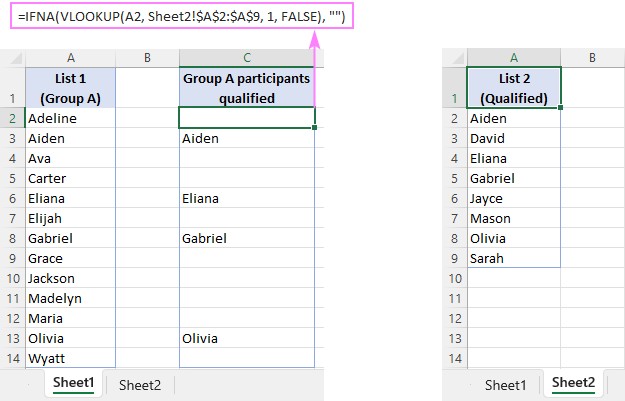
1. Can VLOOKUP compare data in two different Excel files?

Yes, VLOOKUP can compare data in two different Excel files. You need to use the full file path in the table_array argument. For example:

=VLOOKUP(A2, '[Book2.xlsx]Sheet1'!$A$1:$B$10, 2, FALSE)

This formula looks for the value in cell A2 of the current sheet in the range A1:B10 of Sheet1 in Book2.xlsx.

2. How do I compare two columns and return a value from a third column using VLOOKUP?

To compare two columns and return a value from a third column, you can use VLOOKUP with the column containing the return value as the col_index_num. For example:

Product ID	Product Name	Price	Discount
101	Laptop	1200	0.1
102	Keyboard	75	0.05

To find the discount for a specific Product ID, use:

=VLOOKUP(A2, $A$1:$D$10, 4, FALSE)

This formula will return the discount value from the fourth column (Discount) for the Product ID in cell A2.

3. What is the difference between VLOOKUP and XLOOKUP?

VLOOKUP and XLOOKUP are both lookup functions, but XLOOKUP has several advantages:

• Flexibility: XLOOKUP can look to the left, while VLOOKUP can only look to the right.
• Simpler Syntax: XLOOKUP’s syntax is more straightforward, reducing the chance of errors.
• Handles Errors: XLOOKUP has a built-in if_not_found argument to handle errors more gracefully.
• Default Exact Match: XLOOKUP defaults to an exact match, reducing unexpected results.

4. How can I compare two rows and highlight the differences?

You can use conditional formatting to highlight differences between two rows. Select the range of cells you want to compare, then go to Home > Conditional Formatting > New Rule > Use a formula to determine which cells to format. Enter a formula like =A1<>B1 to highlight cells where the values in column A and column B are different.

5. Can I use VLOOKUP to compare text values?

Yes, VLOOKUP can compare text values. Ensure that the text values are consistently formatted (e.g., no leading or trailing spaces) to ensure accurate matches.

6. How do I use VLOOKUP with multiple criteria?

VLOOKUP can’t directly handle multiple criteria. However, you can create a helper column that concatenates the multiple criteria into a single value, then use VLOOKUP on that helper column. For example, if you have columns for Date and Product ID, you can create a helper column with the formula =A2&B2 and use that column for the lookup.

7. How can I improve the performance of VLOOKUP in large datasets?

To improve the performance of VLOOKUP in large datasets:

• Sort the Table Array: Sorting the table array by the lookup column can improve performance.
• Use INDEX and MATCH: INDEX and MATCH can be more efficient than VLOOKUP in some cases.
• Optimize Formulas: Avoid using volatile functions (e.g., NOW(), TODAY()) in your VLOOKUP formulas.
• Use Power Query: For very large datasets, consider using Power Query to load and transform the data.

8. What does the range_lookup argument in VLOOKUP do?

The range_lookup argument in VLOOKUP specifies whether to find an exact match (FALSE) or an approximate match (TRUE). If set to FALSE, VLOOKUP will only return a value if it finds an exact match for the lookup value. If set to TRUE, VLOOKUP will return the closest match that is less than or equal to the lookup value. It’s generally recommended to use FALSE for exact matches to avoid unexpected results.

9. How can I compare two lists and find the differences?

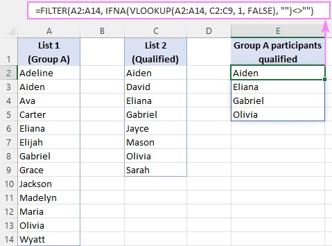
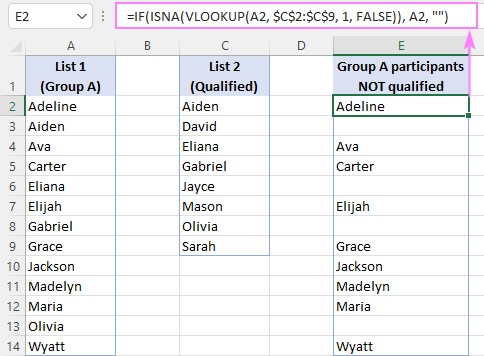
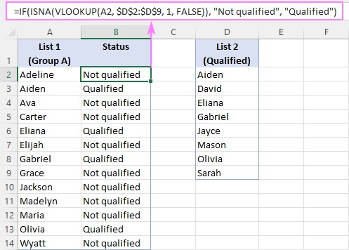
You can use VLOOKUP with the ISNA function to find the differences between two lists. For example:

=IF(ISNA(VLOOKUP(A2, $B$1:$B$10, 1, FALSE)), "Not Found", "Found")

This formula checks if the value in cell A2 is found in the range B1:B10. If it’s not found, the formula returns “Not Found”; otherwise, it returns “Found”.

10. Is VLOOKUP case-sensitive?

No, VLOOKUP is not case-sensitive. It will treat uppercase and lowercase letters as the same. If you need a case-sensitive lookup, you can use more complex formulas involving the EXACT function or consider using Power Query.

Do you find it challenging to compare various products or services? Visit compare.edu.vn at 333 Comparison Plaza, Choice City, CA 90210, United States, or contact us via Whatsapp at +1 (626) 555-9090 to explore our detailed comparison guides.