Comparing two numbers in Excel and identifying differences is straightforward with the right functions and techniques. COMPARE.EDU.VN provides you with the knowledge on essential Excel tools, like formulas and conditional formatting, to master data comparison.
1. What Are the Basic Methods to Compare Two Numbers in Excel?
Excel offers several methods for comparing two numbers, each suited to different scenarios. The basic methods include using formulas with comparison operators, the IF function, and conditional formatting.
1.1 Using Comparison Operators
Comparison operators are the most fundamental way to compare numbers in Excel. These operators include:
=(equal to)>(greater than)<(less than)>=(greater than or equal to)<=(less than or equal to)<>(not equal to)
You can use these operators directly in formulas to compare two numbers. For instance, if you want to check if the value in cell A1 is greater than the value in cell B1, you can use the formula =A1>B1. The result will be TRUE if A1 is indeed greater than B1, and FALSE otherwise.
1.2 Using the IF Function
The IF function is a powerful tool for making comparisons and returning different values based on the outcome. The syntax for the IF function is:
=IF(logical_test, value_if_true, value_if_false)
logical_test: This is the condition you want to evaluate.value_if_true: This is the value that the function returns if the logical test is TRUE.value_if_false: This is the value that the function returns if the logical test is FALSE.
For example, if you want to compare the numbers in cells A1 and B1 and return “Match” if they are equal and “No Match” if they are not, you can use the following formula:
=IF(A1=B1, "Match", "No Match")
1.3 Conditional Formatting
Conditional formatting allows you to highlight cells based on certain criteria. This can be useful for visually identifying differences or matches between numbers.
- Select the cells you want to format.
- Go to Home > Conditional Formatting > New Rule.
- Choose “Use a formula to determine which cells to format.”
- Enter a formula that defines the condition for formatting.
- Click “Format” to choose the formatting style.
For example, to highlight cells in column A that are greater than the corresponding cells in column B, you can use the formula =A1>B1.
2. How Can I Compare Two Columns of Numbers Row by Row?
Comparing two columns of numbers row by row is a common task in Excel. This can be achieved efficiently using formulas and dragging them down the columns.
2.1 Using the IF Function for Row-by-Row Comparison
To compare two columns row by row, you can use the IF function. Suppose you have numbers in columns A and B, and you want to compare them row by row in column C.
- In cell C1, enter the formula
=IF(A1=B1, "Match", "No Match"). - Drag the fill handle (the small square at the bottom-right corner of the cell) down to apply the formula to the rest of the rows.
This will compare the numbers in each row and display “Match” if they are equal and “No Match” if they are not.
2.2 Highlighting Differences with Conditional Formatting
You can also use conditional formatting to highlight differences between two columns row by row.
- Select the range of cells in columns A and B that you want to compare.
- Go to Home > Conditional Formatting > New Rule.
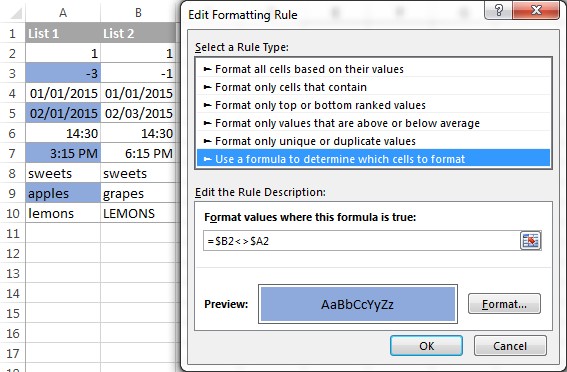
- Choose “Use a formula to determine which cells to format.”
- Enter the formula
=$A1<>$B1to highlight differences. - Click “Format” to choose a highlighting style.
This will highlight the cells where the values in column A are different from the values in column B in the same row.
3. What Formulas Can I Use to Find Differences Between Two Sets of Numbers?
Finding differences between two sets of numbers often involves identifying values that exist in one set but not in the other. Excel provides several formulas to accomplish this.
3.1 Using COUNTIF to Find Unique Values
The COUNTIF function counts the number of cells within a range that meet a given criterion. You can use COUNTIF to find values in one list that do not exist in another.
Suppose you have two lists of numbers in columns A and B. To find the numbers in column A that are not in column B, you can use the following steps:
- In cell C1, enter the formula
=IF(COUNTIF($B:$B, A1)=0, "Unique", ""). - Drag the fill handle down to apply the formula to the rest of the rows in column A.
This formula checks if each value in column A exists in column B. If the count is 0, it means the value is unique to column A, and the formula returns “Unique”.
3.2 Using MATCH and ISNA to Find Differences
The MATCH function searches for a specified item in a range of cells, and then returns the relative position of that item in the range. The ISNA function checks whether a value is the #N/A error value.
- In cell C1, enter the formula
=IF(ISNA(MATCH(A1, $B:$B, 0)), "Unique", ""). - Drag the fill handle down to apply the formula to the rest of the rows in column A.
This formula searches for each value in column A within column B. If MATCH returns #N/A (meaning the value is not found), ISNA returns TRUE, and the IF function returns “Unique”.
3.3 Using the IF Function with the ISERROR and MATCH Functions:
This method is similar to using ISNA and MATCH but uses ISERROR to catch any errors, including #N/A.
In cell C1, enter the formula =IF(ISERROR(MATCH(A1, $B:$B, 0)), “Unique”, “”).
Drag the fill handle down to apply the formula to the rest of the rows in column A.
This formula checks for each value in column A whether it can be found in column B. If MATCH returns an error (meaning the value is not found), ISERROR returns TRUE, and the IF function returns “Unique”.
4. How Can I Highlight Matches and Differences Between Two Lists?
Highlighting matches and differences between two lists can make it easier to visualize and analyze the data. Excel’s conditional formatting feature is ideal for this purpose.
4.1 Highlighting Unique Entries in Each List
To highlight unique entries in each list (i.e., values that appear in only one of the lists), follow these steps:
- Select the first list (e.g., A1:A10).
- Go to Home > Conditional Formatting > New Rule.
- Choose “Use a formula to determine which cells to format.”
- Enter the formula
=COUNTIF($B$1:$B$10, A1)=0to highlight unique values in the first list. - Click “Format” to choose a highlighting style.
- Repeat the steps for the second list (e.g., B1:B10), using the formula
=COUNTIF($A$1:$A$10, B1)=0.
This will highlight the values that are unique to each list.
4.2 Highlighting Matches (Duplicates) Between Two Lists
To highlight matches (duplicates) between two lists, follow these steps:
- Select the first list (e.g., A1:A10).
- Go to Home > Conditional Formatting > New Rule.
- Choose “Use a formula to determine which cells to format.”
- Enter the formula
=COUNTIF($B$1:$B$10, A1)>0to highlight matches in the first list. - Click “Format” to choose a highlighting style.
- Repeat the steps for the second list (e.g., B1:B10), using the formula
=COUNTIF($A$1:$A$10, B1)>0.
This will highlight the values that appear in both lists.
5. How Do I Compare Multiple Columns for Matches in the Same Row?
Comparing multiple columns for matches in the same row is useful when you want to ensure that data across several categories is consistent.
5.1 Using the AND Function
The AND function returns TRUE if all its arguments are TRUE. You can use it to check if multiple columns have the same value in a given row.
For example, if you have data in columns A, B, and C, and you want to check if all three columns have the same value in each row, you can use the following formula in column D:
=IF(AND(A1=B1, A1=C1), "Match", "No Match")
Drag the fill handle down to apply the formula to the rest of the rows.
5.2 Using the COUNTIF Function
The COUNTIF function can also be used to compare multiple columns. If all columns have the same value, the count of any one value across those columns should equal the number of columns.
=IF(COUNTIF($A1:$C1, A1)=3, "Match", "No Match")
Where 3 is the number of columns being compared. Drag the fill handle down to apply the formula to the rest of the rows.
6. How Can I Find the Absolute Difference Between Two Numbers?
Sometimes, you need to find the absolute difference between two numbers, regardless of which number is larger. Excel provides the ABS function for this purpose.
6.1 Using the ABS Function
The ABS function returns the absolute value of a number. To find the absolute difference between two numbers in cells A1 and B1, use the following formula:
=ABS(A1-B1)
This formula calculates the difference between A1 and B1 and then returns the absolute value of that difference.
7. How Do I Compare Two Numbers with a Tolerance?
In many real-world scenarios, you might need to compare two numbers within a certain tolerance. This means considering two numbers as “matching” if their difference is within an acceptable range.
7.1 Using the IF Function with Tolerance
To compare two numbers with a tolerance, you can use the IF function along with the ABS function. Suppose you want to consider two numbers as a match if their absolute difference is less than or equal to 0.1.
=IF(ABS(A1-B1)<=0.1, "Match", "No Match")
This formula checks if the absolute difference between A1 and B1 is less than or equal to 0.1. If it is, the formula returns “Match”; otherwise, it returns “No Match”.
8. How Can I Compare Two Numbers Ignoring Case?
When comparing text-based numbers, you might want to ignore case sensitivity. Excel provides functions to help with this.
8.1 Using the UPPER or LOWER Functions
You can convert both numbers to either uppercase or lowercase and then compare them.
=IF(UPPER(A1)=UPPER(B1), "Match", "No Match")
Or:
=IF(LOWER(A1)=LOWER(B1), "Match", "No Match")
These formulas convert the values in A1 and B1 to uppercase or lowercase, respectively, before comparing them. This ensures that the comparison is case-insensitive.
8.2 Using the EXACT Function for Case-Sensitive Comparison
If you need a case-sensitive comparison, Excel’s EXACT function is useful.
=IF(EXACT(A1, B1), "Match", "No Match")
This formula checks if the values in A1 and B1 are exactly the same, including case. If they match exactly, the formula returns “Match”; otherwise, it returns “No Match”.
9. How Do I Compare Two Numbers and Return the Larger Value?
Sometimes, you simply need to determine which of two numbers is larger. Excel provides the MAX function for this.
9.1 Using the MAX Function
The MAX function returns the largest value in a set of numbers. To compare two numbers in cells A1 and B1 and return the larger value, use the following formula:
=MAX(A1, B1)
This formula returns the larger of the two numbers.
9.2 Using the IF Function to Return the Larger Value
Alternatively, you can use the IF function to return the larger value.
=IF(A1>B1, A1, B1)
This formula checks if A1 is greater than B1. If it is, the formula returns A1; otherwise, it returns B1.
10. How Can I Compare Two Lists and Pull Matching Data?
In many scenarios, you might need to compare two lists and pull matching data from one list to another. Excel provides functions like VLOOKUP, INDEX MATCH, and XLOOKUP for this purpose.
10.1 Using VLOOKUP
VLOOKUP searches for a value in the first column of a range and returns a value in the same row from another column in the range.
=VLOOKUP(D2, $A$2:$B$6, 2, FALSE)
This formula searches for the value in D2 within the range A2:A6 and returns the corresponding value from the second column (column B).
10.2 Using INDEX MATCH
INDEX MATCH is a more flexible alternative to VLOOKUP. It uses the INDEX function to return a value from a specified row and column, and the MATCH function to find the row number.
=INDEX($B$2:$B$6, MATCH($D2, $A$2:$A$6, 0))
This formula searches for the value in D2 within the range A2:A6 and returns the corresponding value from the range B2:B6.
10.3 Using XLOOKUP
XLOOKUP is a more modern function that combines the capabilities of VLOOKUP and INDEX MATCH. It is available in Excel 365 and later versions.
=XLOOKUP(D2, $A$2:$A$6, $B$2:$B$6)
This formula searches for the value in D2 within the range A2:A6 and returns the corresponding value from the range B2:B6.
For more information, please see How to compare two columns using VLOOKUP.
FAQ Section
Q1: How do I compare two cells in Excel to see if they are the same?
To compare two cells in Excel and check if they are the same, you can use a simple IF formula:
=IF(A1=B1, "Same", "Different")
This formula compares the values in cells A1 and B1. If they are the same, it returns “Same”; otherwise, it returns “Different”.
Q2: Can I compare two columns in Excel for partial matches?
Yes, you can compare two columns in Excel for partial matches using functions like SEARCH or FIND combined with the IF function.
=IF(ISNUMBER(SEARCH(A1, B1)), "Partial Match", "No Match")
This formula checks if the value in cell A1 is found within the value in cell B1. If it is, it returns “Partial Match”; otherwise, it returns “No Match”.
Q3: How do I compare two lists and find missing values?
To compare two lists and find missing values, you can use the COUNTIF function or the MATCH function combined with ISNA.
Using COUNTIF:
=IF(COUNTIF($B$1:$B$10, A1)=0, "Missing", "")
Using MATCH and ISNA:
=IF(ISNA(MATCH(A1, $B$1:$B$10, 0)), "Missing", "")
These formulas check if each value in the first list (column A) exists in the second list (column B). If a value is not found, the formula returns “Missing”.
Q4: How can I compare two columns in Excel and return values from a third column?
To compare two columns and return values from a third column, you can use VLOOKUP, INDEX MATCH, or XLOOKUP.
Using VLOOKUP:
=VLOOKUP(A1, $B$1:$C$10, 2, FALSE)
Using INDEX MATCH:
=INDEX($C$1:$C$10, MATCH(A1, $B$1:$B$10, 0))
Using XLOOKUP:
=XLOOKUP(A1, $B$1:$B$10, $C$1:$C$10)
These formulas compare the value in cell A1 with the values in column B and return the corresponding value from column C.
Q5: How do I highlight entire rows based on a comparison between two columns?
To highlight entire rows based on a comparison between two columns, use conditional formatting with a formula that references the first cell in the row.
- Select the entire range of data.
- Go to Home > Conditional Formatting > New Rule.
- Choose “Use a formula to determine which cells to format.”
- Enter the formula
=$A1<>$B1(assuming columns A and B are being compared). - Click “Format” to choose a highlighting style.
This will highlight the entire row where the values in column A are different from the values in column B.
Q6: Can I compare two numbers in different Excel files?
Yes, you can compare two numbers in different Excel files by referencing the cells in the other file in your formulas.
=IF([Book1.xlsx]Sheet1!$A$1=[Book2.xlsx]Sheet1!$A$1, "Match", "No Match")
This formula compares the value in cell A1 of Sheet1 in Book1.xlsx with the value in cell A1 of Sheet1 in Book2.xlsx.
Q7: How do I compare two numbers with different units of measurement?
Comparing two numbers with different units of measurement requires converting them to a common unit first. You can use custom formulas or lookup tables to perform the conversion.
For example, if you have values in meters and feet, you can convert feet to meters using the formula:
=A1 * 0.3048
Then, compare the converted values.
Q8: What is the best way to compare large datasets in Excel?
When comparing large datasets in Excel, consider using techniques that optimize performance, such as:
- Using helper columns with formulas instead of complex array formulas.
- Using conditional formatting sparingly to avoid slowing down Excel.
- Sorting data to group similar values together, which can speed up comparisons.
- Using Excel’s built-in features like “Remove Duplicates” to simplify the data.
- Consider using database software or Excel’s Power Query for extremely large datasets.
Q9: How do I compare two numbers and display the percentage difference?
To compare two numbers and display the percentage difference, use the following formula:
=((B1-A1)/A1)
Format the cell as a percentage to display the result as a percentage.
Q10: Can I use VBA to compare two numbers in Excel?
Yes, you can use VBA (Visual Basic for Applications) to compare two numbers in Excel. Here’s a simple example:
Sub CompareNumbers()
    Dim num1 As Double, num2 As Double
    num1 = Range("A1").Value
    num2 = Range("B1").Value
    If num1 = num2 Then
        MsgBox "The numbers are the same."
    Else
        MsgBox "The numbers are different."
    End If
End Sub
This VBA code compares the values in cells A1 and B1 and displays a message box indicating whether they are the same or different.
Conclusion
Comparing two numbers in Excel involves a variety of techniques, from basic comparison operators and the IF function to more advanced tools like VLOOKUP, INDEX MATCH, and conditional formatting. The methods you choose will depend on the specific requirements of your task. Whether you’re identifying matches, highlighting differences, or pulling matching data, Excel provides the tools you need to analyze your data effectively. Remember, the right approach not only simplifies the process but also enhances the accuracy and efficiency of your analysis. For more detailed guides and tools, visit COMPARE.EDU.VN, your one-stop destination for comprehensive comparisons and informed decision-making.
Need more help in deciding which products or services fit you best? Visit COMPARE.EDU.VN for detailed comparisons that simplify your choices.
Contact us:
Address: 333 Comparison Plaza, Choice City, CA 90210, United States
Whatsapp: +1 (626) 555-9090
Website: compare.edu.vn