Comparing two lists in Excel for differences can be a frequent task for data analysis, and it can be easily done. At COMPARE.EDU.VN, we provide the methods and tools to effectively compare two lists in Excel, highlighting the differences and ensuring accuracy. Streamline your data comparison now. Effortlessly compare lists, identify discrepancies, and maintain data integrity using our user-friendly tutorials. Explore advanced Excel techniques, data analysis strategies, and spreadsheet management tips.
1. What Are The 5 Key Search Intentions For “How To Compare 2 Lists In Excel For Differences?”
Here are the 5 key search intentions for “How To Compare 2 Lists In Excel For Differences”:
- Step-by-step instructions: Users are looking for detailed guides on how to use Excel features and formulas to compare two lists and identify the differences between them.
- Formula examples: Users want specific Excel formulas (e.g., using
COUNTIF,VLOOKUP,MATCH,IF) that they can directly apply to compare lists and highlight or extract the unique entries. - Conditional formatting: Users want to learn how to use conditional formatting to visually highlight the differences between two lists, making it easier to spot discrepancies.
- Tool recommendations: Users are seeking recommendations for Excel add-ins or third-party tools that simplify the process of comparing lists and finding differences, especially when dealing with large datasets.
- Use case scenarios: Users are looking for examples of how to apply list comparison techniques in real-world scenarios, such as identifying missing items in inventory, comparing customer lists, or reconciling financial data.
2. How To Compare Two Columns In Excel Row-By-Row?
To compare two columns in Excel row-by-row, use the IF function to check for matches or differences in each row. This is useful for analyzing data on a per-record basis.
2.1. How To Compare Two Columns For Matches Or Differences In The Same Row?
To compare two columns for matches or differences in the same row, use the IF function to evaluate corresponding cells.
2.1.1. What Is The Formula For Matches?
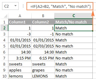
The formula for matches is =IF(A2=B2,"Match",""). This formula checks if the value in cell A2 is equal to the value in cell B2. If they are equal, it returns “Match”; otherwise, it returns an empty string.
2.1.2. What Is The Formula For Differences?
The formula for differences is =IF(A2<>B2,"No match",""). This formula checks if the value in cell A2 is not equal to the value in cell B2. If they are different, it returns “No match”; otherwise, it returns an empty string.
2.1.3. How To Find Matches And Differences In The Same Formula?
To find both matches and differences with a single formula, use =IF(A2=B2,"Match","No match"). This formula returns “Match” if the values in A2 and B2 are equal, and “No match” if they are different.
2.2. How To Compare Two Lists For Case-Sensitive Matches In The Same Row?
To compare two lists for case-sensitive matches in the same row, use the EXACT function within an IF formula. This ensures that the comparison respects the case of the text.
2.2.1. What Is The Formula For Case-Sensitive Matches?
The formula for case-sensitive matches is =IF(EXACT(A2, B2), "Match", ""). The EXACT function compares two text strings and returns TRUE if they are exactly the same, including case. The IF function then returns “Match” if EXACT returns TRUE, and an empty string otherwise.
2.2.2. What Is The Formula For Case-Sensitive Differences?
The formula for case-sensitive differences is =IF(EXACT(A2, B2), "Match", "Unique"). This formula returns “Match” if the values in A2 and B2 are exactly the same (including case), and “Unique” if they are different.
3. How To Compare Multiple Columns For Matches In The Same Row?
To compare multiple columns for matches in the same row, use the AND or COUNTIF functions to check if all or any of the cells have matching values.
3.1. How To Find Matches In All Cells Within The Same Row?
To find matches in all cells within the same row, use an IF formula with an AND statement or the COUNTIF function.
3.1.1. What Is The Formula Using AND?
The formula using AND is =IF(AND(A2=B2, A2=C2), "Full match", ""). This formula checks if the values in A2, B2, and C2 are all equal. If they are, it returns “Full match”; otherwise, it returns an empty string.
3.1.2. What Is The Formula Using COUNTIF?
The formula using COUNTIF is =IF(COUNTIF($A2:$E2, $A2)=5, "Full match", ""). This formula counts how many cells in the range A2:E2 are equal to the value in A2. If the count is 5 (meaning all cells in the range are equal), it returns “Full match”; otherwise, it returns an empty string.
3.2. How To Find Matches In Any Two Cells In The Same Row?
To find matches in any two cells in the same row, use an IF formula with an OR statement or combine multiple COUNTIF functions.
3.2.1. What Is The Formula Using OR?
The formula using OR is =IF(OR(A2=B2, B2=C2, A2=C2), "Match", ""). This formula checks if any of the pairs (A2=B2, B2=C2, A2=C2) are equal. If at least one pair is equal, it returns “Match”; otherwise, it returns an empty string.
3.2.2. How To Combine COUNTIF Functions?
To combine COUNTIF functions, use a formula like =IF(COUNTIF(B2:D2,A2)+COUNTIF(C2:D2,B2)+(C2=D2)=0,"Unique","Match"). This formula checks if there are any matches between the specified columns. If no matches are found, it returns “Unique”; otherwise, it returns “Match”.
4. How To Compare Two Columns In Excel For Matches And Differences?
To compare two columns in Excel for matches and differences, use the COUNTIF function within an IF formula to check if values in one column exist in another.
4.1. What Is The Formula To Find Values In Column A That Are Not In Column B?
The formula to find values in column A that are not in column B is =IF(COUNTIF($B:$B, $A2)=0, "No match in B", ""). This formula checks if the value in cell A2 exists in column B. If COUNTIF returns 0 (meaning no match is found), the formula returns “No match in B”; otherwise, it returns an empty string.
4.2. What Is The Formula Using ISERROR And MATCH?
The formula using ISERROR and MATCH is =IF(ISERROR(MATCH($A2,$B$2:$B$10,0)),"No match in B",""). This formula uses the MATCH function to find the position of the value in A2 within the range B2:B10. If MATCH returns an error (meaning the value is not found), ISERROR returns TRUE, and the IF function returns “No match in B”; otherwise, it returns an empty string.
4.3. How To Use An Array Formula?
To use an array formula, enter =IF(SUM(--($B$2:$B$10=$A2))=0, "No match in B", "") and press Ctrl + Shift + Enter. This formula compares the value in A2 with each value in the range B2:B10. If the sum of the matches is 0 (meaning no match is found), the formula returns “No match in B”; otherwise, it returns an empty string.
4.4. How To Identify Both Matches And Differences In A Single Formula?
To identify both matches and differences in a single formula, use =IF(COUNTIF($B:$B, $A2)=0, "No match in B", "Match in B"). This formula returns “No match in B” if the value in A2 is not found in column B, and “Match in B” if it is found.
5. How To Compare Two Lists In Excel And Pull Matches?
To compare two lists in Excel and pull matches, use functions like VLOOKUP, INDEX MATCH, or XLOOKUP to retrieve corresponding data from one list based on matches in another.
5.1. How To Use VLOOKUP?
To use VLOOKUP, the formula is =VLOOKUP(D2, $A$2:$B$6, 2, FALSE). This formula searches for the value in D2 within the range A2:A6, and if a match is found, it returns the corresponding value from the second column of the range (column B).
5.2. How To Use INDEX MATCH?
To use INDEX MATCH, the formula is =INDEX($B$2:$B$6, MATCH($D2, $A$2:$A$6, 0)). This formula first uses MATCH to find the position of the value in D2 within the range A2:A6, and then uses INDEX to return the value from the corresponding position in the range B2:B6.
5.3. How To Use XLOOKUP?
To use XLOOKUP, the formula is =XLOOKUP(D2, $A$2:$A$6, $B$2:$B$6). This formula searches for the value in D2 within the range A2:A6, and if a match is found, it returns the corresponding value from the range B2:B6.
6. How To Compare Two Lists And Highlight Matches And Differences?
To compare two lists and highlight matches and differences, use Excel’s Conditional Formatting feature to visually identify unique or duplicate entries.
6.1. How To Highlight Matches And Differences In Each Row?
To highlight matches and differences in each row, use Conditional Formatting with formulas that check for equality or inequality between cells.
6.1.1. How To Highlight Identical Entries?
To highlight identical entries, select the cells, go to Conditional Formatting > New Rule > Use a formula to determine which cells to format, and enter the formula =$B2=$A2.
6.1.2. How To Highlight Differences?
To highlight differences, select the cells, go to Conditional Formatting > New Rule > Use a formula to determine which cells to format, and enter the formula =$B2<>$A2.
6.2. How To Highlight Unique Entries In Each List?
To highlight unique entries in each list, use Conditional Formatting with COUNTIF to identify values that appear only in one list.
6.2.1. How To Highlight Unique Values In List 1 (Column A)?
To highlight unique values in List 1 (column A), use the formula =COUNTIF($C$2:$C$5, $A2)=0.
6.2.2. How To Highlight Unique Values In List 2 (Column C)?
To highlight unique values in List 2 (column C), use the formula =COUNTIF($A$2:$A$6, $C2)=0.
6.3. How To Highlight Matches (Duplicates) Between Two Columns?
To highlight matches (duplicates) between two columns, use Conditional Formatting with COUNTIF to identify values that appear in both lists.
6.3.1. How To Highlight Matches In List 1 (Column A)?
To highlight matches in List 1 (column A), use the formula =COUNTIF($C$2:$C$5, $A2)>0.
6.3.2. How To Highlight Matches In List 2 (Column C)?
To highlight matches in List 2 (column C), use the formula =COUNTIF($A$2:$A$6, $C2)>0.
7. How To Highlight Row Differences And Matches In Multiple Columns?
To highlight row differences and matches in multiple columns, use Conditional Formatting for matches and Excel’s Go To Special feature for differences.
7.1. How To Compare Multiple Columns And Highlight Row Matches?
To highlight rows with identical values in all columns, use Conditional Formatting with formulas like AND or COUNTIF.
7.1.1. What Is The Formula Using AND?
The formula using AND is =AND($A2=$B2, $A2=$C2).
7.1.2. What Is The Formula Using COUNTIF?
The formula using COUNTIF is =COUNTIF($A2:$C2, $A2)=3.
7.2. How To Compare Multiple Columns And Highlight Row Differences?
To quickly highlight cells with different values in each individual row, use Excel’s Go To Special feature.
- Select the range of cells.
- Go to Home > Editing > Find & Select > Go To Special…
- Select Row differences and click OK.
- Shade the highlighted cells using the Fill Color icon.
8. How To Compare Two Cells In Excel?
To compare two cells in Excel, use the IF function to check for matches or differences.
8.1. What Is The Formula For Matches?
The formula for matches is =IF(A1=C1, "Match", "").
8.2. What Is The Formula For Differences?
The formula for differences is =IF(A1<>C1, "Difference", "").
 Compare two cells in Excel for matches.
9. What Is A Formula-Free Way To Compare Two Columns / Lists In Excel?
A formula-free way to compare two columns/lists in Excel is by using add-ins like Compare Two Tables from Ablebits Ultimate Suite. This tool simplifies the process by identifying and highlighting matches and differences without needing formulas.
9.1. How To Use Compare Two Tables Add-In?
To use the Compare Two Tables add-in:
- Click the Compare Tables button on the Ablebits Data tab.
- Select the first column/list (Table 1) and click Next.
- Select the second column/list (Table 2) and click Next.
- Choose to look for Duplicate values (matches) or Unique values (differences).
- Select the columns for comparison.
- Choose how to deal with the found items: Highlight with color or Identify in the Status column, and click Finish.
10. What Are Some FAQs About Comparing Two Lists In Excel For Differences?
Here are some frequently asked questions about comparing two lists in Excel for differences:
10.1. Can I Compare Two Lists In Different Worksheets?
Yes, you can compare two lists in different worksheets by referencing the correct sheet names in your formulas or by using add-ins that support cross-sheet comparisons. For example, using a formula like =IF(Sheet1!A1=Sheet2!A1, "Match", "No Match") to compare corresponding cells in Sheet1 and Sheet2.
10.2. How Do I Handle Case Sensitivity When Comparing Lists?
To handle case sensitivity, use the EXACT function within your formulas. For instance, use =IF(EXACT(A1, B1), "Match", "No Match") to ensure the comparison is case-sensitive.
10.3. What Is The Best Way To Compare Large Lists In Excel?
For large lists, using array formulas or the COUNTIF function can be computationally intensive. Consider using Excel’s built-in filtering and sorting features, or opt for specialized Excel add-ins designed for comparing large datasets efficiently, such as Power Query or the Ablebits Ultimate Suite.
10.4. How Can I Compare Two Lists And Return The Values That Are Different?
You can use the IF and COUNTIF functions to compare two lists and return the values that are different. For example, to find values in List A that are not in List B, use the formula =IF(COUNTIF(ListB_Range, A1)=0, A1, "").
10.5. Is It Possible To Compare Two Lists And Highlight The Entire Row Based On A Match?
Yes, you can highlight the entire row based on a match by using conditional formatting with a formula that references a specific column for the match condition. For example, select the entire range of rows you want to format, then create a new conditional formatting rule using the formula =$A1=B$1 (assuming column A in your selected range is where you are checking for the match).
10.6. How Do I Ignore Blank Cells When Comparing Two Lists?
To ignore blank cells, you can add an additional condition to your IF formulas to check if the cells are not blank. For example, use =IF(AND(A1<>"", B1<>""), IF(A1=B1, "Match", "No Match"), "") to compare A1 and B1 only if both cells are not blank.
10.7. Can I Compare Two Lists Based On Partial Matches?
Yes, you can compare two lists based on partial matches by using functions like SEARCH or FIND within your formulas. For example, use =IF(ISNUMBER(SEARCH(B1, A1)), "Partial Match", "No Match") to check if the value in B1 is a substring of the value in A1.
10.8. How Do I Compare Two Lists And Return The Number Of Differences?
To return the number of differences between two lists, you can use a combination of SUM and IF functions in an array formula. For example, use =SUM(IF(A1:A10<>B1:B10, 1, 0)) entered as an array formula (Ctrl+Shift+Enter) to count the number of cells in the range A1:A10 that are different from the corresponding cells in B1:B10.
10.9. What Are Some Common Mistakes To Avoid When Comparing Lists In Excel?
Some common mistakes to avoid include:
- Not using absolute references (
$) when necessary, which can cause formulas to return incorrect results when copied. - Forgetting to handle case sensitivity when comparing text values.
- Not accounting for blank cells or errors in your formulas.
- Using inefficient methods for large datasets, which can slow down Excel and make it unresponsive.
10.10. Can I Automate The List Comparison Process In Excel?
Yes, you can automate the list comparison process by using VBA (Visual Basic for Applications) macros. You can write VBA code to loop through the lists, compare values, and perform actions based on the comparison results. This can be especially useful for repetitive tasks or complex comparison scenarios.
By using these formulas, techniques, and tools, you can effectively compare two lists in Excel for differences, ensuring accuracy and efficiency in your data analysis tasks.
Ready to take your Excel skills to the next level? Visit COMPARE.EDU.VN today to discover more ways to compare and analyze data, streamline your decision-making process, and stay ahead of the curve. Our comprehensive guides and expert tips are designed to help you make informed choices, whether you’re comparing products, services, or educational opportunities.
Don’t miss out on the opportunity to make smarter decisions. Visit COMPARE.EDU.VN now and unlock the power of informed comparisons.
Address: 333 Comparison Plaza, Choice City, CA 90210, United States
Whatsapp: +1 (626) 555-9090
Website: compare.edu.vn