**How To Compare 2 Columns In Excel For Duplicates?**

Comparing two columns in Excel for duplicates is made simple with several techniques, and COMPARE.EDU.VN is here to guide you through them. This article will explore various methods, including conditional formatting, using the equals operator, VLOOKUP, IF formulas, and the EXACT function, to help you identify matching and unique entries. By mastering these methods, you can efficiently manage and analyze your data in Excel, optimizing your workflow for data cleaning, auditing, and reporting.

1. What Does Comparing Columns in Excel Mean?

Comparing columns in Excel involves checking cells across different columns to find similarities and differences. This process is essential for identifying duplicate entries, inconsistencies, or unique values within your data. By systematically comparing columns, you can ensure data accuracy, identify trends, and make informed decisions. This action often includes flagging matching data points or pinpointing those lacking corresponding entries.

2. How to Compare Two Columns in Excel?

There are several effective methods for comparing two columns in Excel, each with its strengths and use cases. These methods include:

Conditional Formatting
Equals Operator
VLOOKUP Function
IF Formula
EXACT Formula

Let’s explore each of these methods in detail to help you choose the best one for your specific needs.

2.1. Using Conditional Formatting in Excel

Conditional formatting in Excel is a straightforward way to highlight duplicate or unique values in two columns. It allows you to visually identify matching or non-matching entries quickly.

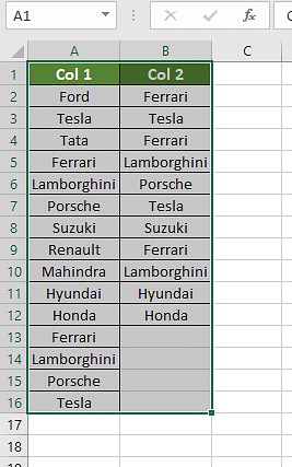
2.1.1. Step 1: Selecting the Cells

Start by selecting all the cells in the spreadsheet that you want to compare.

2.1.2. Step 2: Applying Conditional Formatting

Navigate to the “Home” tab, find the “Conditional Formatting” option in the toolbar, and select “Highlight Cells Rules,” then choose “Duplicate Values.”

2.1.3. Step 3: Choosing Duplicate or Unique Values

A new window will appear, allowing you to select either “Duplicate” or “Unique” values. Choose the option that suits your comparison needs. Selecting “Duplicate” will highlight all matching entries, while selecting “Unique” will highlight entries that appear only once in your selected columns.

2.1.3.1. Highlighting Duplicate Values

If you choose “Duplicate” values, Excel will highlight all the cells that have matching entries in the selected columns.

2.1.3.2. Highlighting Unique Values

If you choose “Unique” values, Excel will highlight all the cells that have unique entries in the selected columns.

2.2. Using the Equals Operator

Another simple method for comparing columns in Excel is using the equals operator (=). This method allows you to create a new column that displays whether the values in two corresponding cells are the same (TRUE) or different (FALSE).

2.2.1. Step 1: Creating a Result Column

Create a new column next to the columns you want to compare. In the first cell of this new column, enter a formula that compares the corresponding cells in the other two columns. For example, if you are comparing column A and column B, the formula in the first cell of the new column (e.g., C2) would be “=A2=B2”.

2.2.2. Step 2: Applying the Formula

Drag the fill handle (the small square at the bottom right of the cell) down to apply the formula to all the rows you want to compare. Excel will display “TRUE” for each row where the values in the two columns match and “FALSE” where they differ.

2.2.3. Step 3: Customizing the Output (Optional)

You can customize the output to display more descriptive messages instead of “TRUE” and “FALSE.” Use the IF function to specify custom messages for matching and non-matching values. For example, the formula could be “=IF(A2=B2, “Match”, “No Match”)”.

2.3. Using the VLOOKUP Function

The VLOOKUP function is useful for comparing two columns in Excel, especially when you need to find matches and retrieve corresponding data from one column to another. This method is particularly effective when you want to check if values from one column exist in another.

2.3.1. Understanding the VLOOKUP Formula

The VLOOKUP formula has the following syntax:

=VLOOKUP(lookup_value, table_array, col_index_num, [range_lookup])

lookup_value: The value you want to search for in the first column of the table array.
table_array: The range of cells that contains the data you want to search.
col_index_num: The column number in the table array from which to return a value if a match is found.
[range_lookup]: Optional. Specify TRUE for an approximate match (the first column in the table array should be sorted in ascending order) or FALSE for an exact match. Generally, use FALSE for comparing columns.

2.3.2. Step 1: Setting Up the Formula

Create a new result column and add the VLOOKUP formula to compare individual cells. For instance, if you want to check if values in column A exist in column B, the formula in the new column (e.g., C2) would be “=VLOOKUP(A2, B:B, 1, FALSE)”. Here, A2 is the lookup value (the value from column A that you want to find), B:B is the table array (column B, where you are searching for the value), 1 is the column index number (since we are looking in only one column, it’s 1), and FALSE specifies that you want an exact match.

2.3.3. Step 2: Applying the Formula

Drag the formula down to apply it to all the cells in the result column. If a value from column A is found in column B, VLOOKUP will return that value. If the value is not found, VLOOKUP will return an error (#N/A).

2.3.4. Step 3: Handling Errors (Optional)

To handle errors (e.g., #N/A), you can use the IFERROR function. This function allows you to display a custom message when VLOOKUP doesn’t find a match. For example, the modified formula could be “=IFERROR(VLOOKUP(A2, B:B, 1, FALSE), “Not Found”)”. This will display “Not Found” in the result column for any value in column A that does not exist in column B.

2.3.5. Step 4: Addressing Partial Matches with Wildcards (Optional)

In some cases, the values you are comparing might not be exactly the same. For example, one column might contain “Ford India,” while the other contains “Ford.” To address these partial matches, you can use wildcards in the VLOOKUP formula. For example, the modified formula could be “=IFERROR(VLOOKUP(A2&”“, B:B, 1, FALSE), “Not Found”)”. The asterisk () acts as a wildcard, allowing VLOOKUP to find values in column B that start with the value in column A.

2.4. Comparing Two Columns Using the IF Formula

The IF formula in Excel is a powerful tool for comparing two columns, allowing you to specify different results based on whether the values match or differ. This method is useful when you want to display custom messages or perform different calculations depending on the comparison.

2.4.1. Understanding the IF Formula

The IF formula has the following syntax:

=IF(logical_test, value_if_true, value_if_false)

logical_test: The condition you want to evaluate (e.g., A2=B2).
value_if_true: The value to return if the logical test is TRUE.
value_if_false: The value to return if the logical test is FALSE.

2.4.2. Step 1: Setting Up the Formula

In a new result column, enter the IF formula to compare the corresponding cells in the two columns. For example, if you are comparing column A and column B and want to display “Match” if the values are the same and “Different” if they are not, the formula in the first cell of the new column (e.g., C2) would be “=IF(A2=B2, “Match”, “Different”)”.

2.4.3. Step 2: Applying the Formula

Drag the fill handle down to apply the formula to all the rows you want to compare. Excel will display “Match” for each row where the values in the two columns are the same and “Different” where they differ.

2.5. Comparing Using the EXACT Formula

The EXACT formula in Excel is used to compare two values, ensuring that the comparison is case-sensitive. This means that “Apple” and “apple” would be considered different. The EXACT formula is particularly useful when you need to ensure that the values are exactly the same, including case, spaces, and other characters.

2.5.1. Understanding the EXACT Formula

The EXACT formula has the following syntax:

=EXACT(text1, text2)

text1: The first text string to compare.
text2: The second text string to compare.

The formula returns TRUE if the two text strings are exactly the same (including case) and FALSE if they are not.

2.5.2. Step 1: Setting Up the Formula

In a new result column, enter the EXACT formula to compare the corresponding cells in the two columns. For example, if you are comparing column A and column B, the formula in the first cell of the new column (e.g., C2) would be “=EXACT(A2, B2)”.

2.5.3. Step 2: Applying the Formula

Drag the fill handle down to apply the formula to all the rows you want to compare. Excel will display “TRUE” for each row where the values in the two columns are exactly the same (including case) and “FALSE” where they differ.

3. Which Method Should You Use?

Choosing the right method for comparing two columns in Excel depends on the specific scenario and what you need to achieve. Here’s a guide to help you decide.

3.1. Scenario 1: Comparing Two Columns Row-by-Row

When you need to compare two columns in Excel row-by-row and display a result for each row, use the following formulas:

=IF(A2 = B2, “Match”, ” “): This formula returns “Match” if the values in A2 and B2 are the same and a blank space if they are different.
=IF(A2<>B2, “No Match”, ” “): This formula returns “No Match” if the values in A2 and B2 are different and a blank space if they are the same.
=IF(A2 = B2, “Match”, “No Match”): This formula returns “Match” if the values in A2 and B2 are the same and “No Match” if they are different.

If you need the results to be case-sensitive, use the EXACT formula within the IF formula:

=IF(EXACT(A2, B2), “Match”, ” “): This formula returns “Match” if the values in A2 and B2 are exactly the same (including case) and a blank space if they are different.
=IF(EXACT(A2, B2), “Match”, “No Match”): This formula returns “Match” if the values in A2 and B2 are exactly the same (including case) and “No Match” if they are different.

3.2. Scenario 2: Comparing Multiple Columns for Row Matches

If you need to compare more than two columns to find similarities and differences, use the following formulas:

=IF(AND(A2=B2, A2=C2), “Complete Match”, ” “): This formula returns “Complete Match” if the values in A2, B2, and C2 are all the same and a blank space if they are not.
=IF(COUNTIF($A2:$E2, $A2)=4, “Complete Match”, ” “): This formula returns “Complete Match” if the value in A2 appears 4 times in the range A2 to E2. Adjust the number 4 to match the number of columns you are comparing.

To compare columns and identify rows with any two or more cells having the same values, use:

=IF(OR(A2=B2, B2=C2, A2=C2), “Match”, “”): This formula returns “Match” if any two of the values in A2, B2, and C2 are the same and a blank space if they are all different.
=IF(COUNTIF(B2:D2,A2)+COUNTIF(C2:D2,B2)+(C2=D2)=0,”Unique”,”Match”): This formula returns “Unique” if all the values in A2, B2, and C2 are different and “Match” if any two are the same.

3.3. Scenario 3: Compare Two Columns for Matches and Differences

To compare two datasets and find unique values present in column A but not in column B, use the following formulas:

=IF(COUNTIF($B:$B, $A2)=0, “Not Present in B”, “”): This formula returns “Not Present in B” if the value in A2 does not appear in column B and a blank space if it does.
=IF(ISERROR(MATCH($A2,$B$2:$B$10,0)),”Not Present in B”,””): This formula returns “Not Present in B” if the value in A2 does not appear in the range B2 to B10 and a blank space if it does.

To get a result for both matches and unique values, use:

=IF(COUNTIF($B:$B, $A2)=0, “Not Present in B”, “Present in B”): This formula returns “Not Present in B” if the value in A2 does not appear in column B and “Present in B” if it does.

3.4. Scenario 4: Compare Two Lists and Pull Matching Data

To compare two lists and find matching data, you can use the VLOOKUP function or the INDEX MATCH formula. Here are the formulas for this scenario:

=VLOOKUP(D2, $A$2:$B$6, 2, FALSE): This formula looks for the value in D2 in the range A2:A6 and returns the corresponding value from column B. If the value is not found, it returns an error.
=INDEX($B$2:$B$6, MATCH($D2, $A$2:$A$6, 0)): This formula finds the position of the value in D2 in the range A2:A6 and returns the corresponding value from the range B2:B6. If the value is not found, it returns an error.
=XLOOKUP(D2, $A$2:$A$6, $B$2:$B$6): This formula looks for the value in D2 in the range A2:A6 and returns the corresponding value from the range B2:B6. XLOOKUP is a newer function and is available in Excel 365 and later versions.

3.5. Scenario 5: Highlight Row Matches and Differences

You can create a conditional formatting formula to highlight rows that include identical values in all columns. Use the following formulas for this purpose:

=AND($A2=$B2, $A2=$C2): This formula returns TRUE if the values in A2, B2, and C2 are all the same and FALSE if they are not.
=COUNTIF($A2:$C2, $A2)=3: This formula returns TRUE if the value in A2 appears 3 times in the range A2 to C2, indicating that all three values are the same.

To highlight the matches and differences, follow these steps:

Select the columns with the dataset you want to compare.
Go to the “Home” tab, click on “Conditional Formatting,” select “New Rule,” and choose “Use a formula to determine which cells to format.”
Enter one of the formulas above in the formula box.
Click on “Format” and choose the formatting style you want to apply to the matching rows.
Click “OK” to apply the conditional formatting.

Alternatively, you can use the “Go To Special” option to find and highlight differences:

Select the columns with the dataset you want to compare.
Go to the “Home” tab, click “Find & Select” in the “Editing” group, and choose “Go To Special.”
Select “Row Differences” and click “OK.”
The cells with different values in each row will be selected. You can then change the fill color to highlight the differences.

4. Frequently Asked Questions

4.1. How Do I Compare Two Columns in Excel?

One popular method for comparing two columns in Excel involves selecting both columns of data, navigating to the “Home” tab, clicking on “Find & Select,” choosing “Go To Special,” selecting “Row Differences,” and then clicking “OK.” This method highlights the cells with differing values in each row.

4.2. Can I Compare Two Columns in Excel Using the Index-Match Function?

Yes, you can compare two columns in Excel using the Index-Match function. This involves creating a formula that utilizes the Index and Match functions to find matching values between the two columns. The Index function returns a value from a specified range, while the Match function finds the position of a value within a range.

4.3. How Can I Compare Multiple Columns in Excel?

To compare multiple columns in Excel, you can use the conditional formatting option on the “Home” tab. Format the setting to highlight “duplicates” or “uniques,” and choose a desired color to highlight the values for comparison across multiple columns. This visual method helps in quickly identifying matching or unique entries across several columns.

4.4. How Do You Compare Two Lists in Excel for Matches?

You can compare two lists in Excel using the IF function, MATCH function, or highlighting row differences. The IF function allows you to specify a condition (e.g., A2=B2) and return a value based on whether the condition is true or false. The MATCH function finds the position of a value in a list, and highlighting row differences helps visually identify matching or differing entries.

4.5. How Do I Compare Two Columns in Excel and Highlight the Duplicates?

To compare two columns in Excel and highlight the duplicates, follow these steps:

Select the two columns you want to compare.
Go to the “Home” tab and click on “Conditional Formatting.”
Choose “Highlight Cells Rules” and select “Duplicate Values” from the dropdown menu.
In the “Duplicate Values” dialog box, ensure “Duplicate” is selected.
Choose a formatting style or leave the default style.
Click “OK.”

Excel will then highlight the duplicate values in the selected columns, making them easy to identify.

5. Conclusion

Comparing two columns in Excel for duplicates is an essential skill for data analysis and management. Whether you’re using conditional formatting, the equals operator, VLOOKUP, IF formulas, or the EXACT function, each method offers a unique approach to identifying matching and unique entries. At COMPARE.EDU.VN, we understand the importance of efficient data handling, and these techniques are designed to streamline your workflow, ensuring accuracy and informed decision-making.

For more in-depth comparisons and detailed guides on various topics, be sure to visit COMPARE.EDU.VN. We are dedicated to providing comprehensive and objective comparisons to help you make the best choices. Contact us at 333 Comparison Plaza, Choice City, CA 90210, United States, or reach out via WhatsApp at +1 (626) 555-9090. Explore our website at compare.edu.vn for more information.