Comparing two columns in Excel to identify similarities and differences can be a time-consuming task. Compare.edu.vn offers multiple solutions to streamline this process, from using formulas to employing conditional formatting, ensuring accuracy and efficiency. Leverage Excel’s capabilities to enhance your data analysis skills with various comparison techniques, or discover a faster and intuitive solution using third party tools. Master Excel comparisons and data matching.
1. Comparing Two Columns Row-by-Row in Excel
When working with data analysis in Excel, comparing data within each individual row is a frequent requirement. This can be effectively achieved using the IF function.
1.1. Comparing Two Columns for Matches or Differences in the Same Row
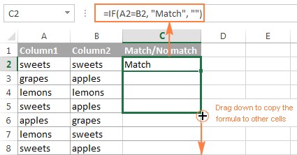
To compare two columns in Excel on a row-by-row basis, you can use a simple IF formula that compares the first two cells. Enter the formula in a separate column within the same row, and then drag the fill handle (the small square at the bottom-right corner of the selected cell) down to apply it to the remaining cells.
1.1.1. Formula for Matches
To identify cells within the same row that contain identical content, you can use the following formula, assuming that the cells to be compared are A2 and B2:
=IF(A2=B2,"Match","")
1.1.2. Formula for Differences
To find cells in the same row that have different values, replace the equals sign (=) with the not equal to sign (<>):
=IF(A2<>B2,"No match","")
1.1.3. Matches and Differences
You can also combine both matches and differences into a single formula:
=IF(A2=B2,"Match","No match")
Or
=IF(A2<>B2,"No match","Match")
The result might look like this:
The formula works effectively with numbers, dates, times, and text strings.
Tip: You can also compare two columns row-by-row using Excel’s Advanced Filter. This allows you to filter for matches and differences between two columns.
1.2. Comparing Two Lists for Case-Sensitive Matches in the Same Row
The previous examples ignore case sensitivity when comparing text values. To find case-sensitive matches between two columns in each row, use the EXACT function:
=IF(EXACT(A2, B2), "Match", "")
To identify case-sensitive differences in the same row, enter the appropriate text (e.g., “Unique”) in the third argument of the IF function:
=IF(EXACT(A2, B2), "Match", "Unique")
2. Comparing Multiple Columns for Matches in the Same Row
In Excel worksheets, multiple columns can be compared based on specific criteria.
2.1. Finding Matches in All Cells Within the Same Row
If the table has three or more columns and you want to find rows with the same values in all cells, use an IF formula with an AND statement:
=IF(AND(A2=B2, A2=C2), "Full match", "")
For tables with numerous columns, use the COUNTIF function:
=IF(COUNTIF($A2:$E2, $A2)=5, "Full match", "")
Where 5 represents the number of columns being compared.
2.2. Finding Matches in Any Two Cells in the Same Row
To compare columns for any two or more cells with the same values within the same row, use an IF formula with an OR statement:
=IF(OR(A2=B2, B2=C2, A2=C2), "Match", "")
If there are many columns, an OR statement might become too large. In this case, use multiple COUNTIF functions. The first COUNTIF counts how many columns have the same value as in the first column, the second COUNTIF counts how many of the remaining columns are equal to the second column, and so on. If the count is 0, the formula returns “Unique”; otherwise, it returns “Match.” For example:
=IF(COUNTIF(B2:D2,A2)+COUNTIF(C2:D2,B2)+(C2=D2)=0,"Unique","Match")
3. Comparing Two Columns in Excel for Matches and Differences
To find values (numbers, dates, or text strings) that are in column A but not in column B, embed the COUNTIF($B:$B, $A2)=0 function in IF’s logical test to check if it returns zero (no match) or any other number (at least one match).
For example, the following IF/COUNTIF formula searches across column B for the value in cell A2. If no match is found, the formula returns “No match in B”; otherwise, it returns an empty string:
=IF(COUNTIF($B:$B, $A2)=0, "No match in B", "")
Tip: If the table has a fixed number of rows, specify a range (e.g., $B2:$B10) rather than the entire column ($B:$B) for the formula to work faster on large datasets.
The same result can be achieved using an IF formula with the embedded ISERROR and MATCH functions:
=IF(ISERROR(MATCH($A2,$B$2:$B$10,0)),"No match in B","")
Alternatively, use this array formula (press Ctrl + Shift + Enter to enter it correctly):
=IF(SUM(--($B$2:$B$10=$A2))=0, " No match in B", "")
To identify both matches (duplicates) and differences (unique values) with a single formula, enter text for matches in the empty double quotes (“”) in any of the above formulas. For example:
=IF(COUNTIF($B:$B, $A2)=0, "No match in B", "Match in B")
4. Comparing Two Lists in Excel and Pulling Matches
To not only match two columns in different tables but also pull matching entries from the lookup table, Excel provides the VLOOKUP function. As an alternative, use the INDEX MATCH formula or, for Excel 2021 and Excel 365 users, the XLOOKUP function.
For example, the following formulas compare product names in column D against names in column A and pull a corresponding sales figure from column B if a match is found; otherwise, the #N/A error is returned.
=VLOOKUP(D2, $A$2:$B$6, 2, FALSE)
=INDEX($B$2:$B$6, MATCH($D2, $A$2:$A$6, 0))
=XLOOKUP(D2, $A$2:$A$6, $B$2:$B$6)
5. Comparing Two Lists and Highlighting Matches and Differences
To visually identify items that are present in one column but missing in another, use Excel’s Conditional Formatting feature to shade such cells.
5.1. Highlighting Matches and Differences in Each Row
To compare two columns in Excel and highlight cells in column A with identical entries in column B in the same row, follow these steps:
- Select the cells to highlight.
- Click Conditional formatting > New Rule… > Use a formula to determine which cells to format.
- Create a rule with a formula like
=$B2=$A2(assuming row 2 is the first row with data, excluding the column header). Ensure a relative row reference (without the $ sign) is used.
To highlight differences between columns A and B, create a rule with this formula:
=$B2<>$A2
5.2. Highlighting Unique Entries in Each List
When comparing two lists in Excel, highlight items that are only in the first list (unique), items that are only in the second list (unique), and items that are in both lists (duplicates).
To color items that are only in one list, assuming List 1 is in column A (A2:A6) and List 2 is in column C (C2:C5), create conditional formatting rules with these formulas:
Highlight unique values in List 1 (column A):
=COUNTIF($C$2:$C$5, $A2)=0
Highlight unique values in List 2 (column C):
=COUNTIF($A$2:$A$6, $C2)=0
This will result in:
5.3. Highlighting Matches (Duplicates) Between Two Columns
Adjust the COUNTIF formulas to find matches rather than differences by setting the count greater than zero:
Highlight matches in List 1 (column A):
=COUNTIF($C$2:$C$5, $A2)>0
Highlight matches in List 2 (column C):
=COUNTIF($A$2:$A$6, $C2)>0
6. Highlighting Row Differences and Matches in Multiple Columns
When comparing values in several columns row-by-row, the quickest way to highlight matches is by creating a conditional formatting rule, and the fastest way to shade differences is by using the Go To Special feature.
6.1. Comparing Multiple Columns and Highlighting Row Matches
To highlight rows that have identical values in all columns, create a conditional formatting rule based on one of these formulas:
=AND($A2=$B2, $A2=$C2)
or
=COUNTIF($A2:$C2, $A2)=3
Where A2, B2, and C2 are the top-most cells, and 3 is the number of columns to compare.
These formulas can be adjusted to compare more than three columns.
6.2. Comparing Multiple Columns and Highlighting Row Differences
To quickly highlight cells with different values in each individual row, use Excel’s Go To Special feature.
- Select the range of cells to compare. The top-most cell of the selected range is the active cell, and the cells from the other selected columns in the same row will be compared to that cell.
- To change the comparison column, use the Tab key to navigate through selected cells from left to right, or the Enter key to move from top to bottom.
- On the Home tab, go to Editing group, and click Find & Select > Go To Special… Then select Row differences and click the OK button.
- The cells whose values are different from the comparison cell in each row are colored. To shade the highlighted cells in a specific color, click the Fill Color icon on the ribbon and select the desired color.
7. Comparing Two Cells in Excel
Comparing two cells is a particular case of comparing two columns in Excel row-by-row, except you don’t have to copy the formulas down to other cells in the column.
For example, to compare cells A1 and C1, use the following formulas:
For matches:
=IF(A1=C1, "Match", "")
For differences:
=IF(A1<>C1, "Difference", "")
8. Formula-Free Way to Compare Two Columns/Lists in Excel
Third-party tools like Ablebits Ultimate Suite offer a solution for comparing and matching columns. This add-in can compare two tables or lists by any number of columns and identify matches/differences and highlight them.
To compare two lists using this tool, follow these steps:
- Click the Compare Tables button on the Ablebits Data tab.
- Select the first column/list and click Next.
- Select the second column/list and click Next.
- Choose what kind of data to look for:
- Duplicate values (matches) – the items that exist in both lists.
- Unique values (differences) – the items that are present in list 1, but not in list 2.
- Select the columns for comparison.
- Choose how to deal with the found items and click Finish. Options include:
- Highlight with color – shades matches or differences in the selected color (like Excel conditional formatting does).
- Identify in the Status column – inserts the Status column with the “Duplicate” or “Unique” labels (like IF formulas do).
For example, highlighting duplicates would result in:
With the Status column, the result would look like this:
FAQ Section
8.1. How do I compare two columns in Excel for exact matches?
Use the EXACT function within an IF statement to compare two columns for case-sensitive matches. For example: =IF(EXACT(A2, B2), "Match", "No Match").
8.2. Can I compare two columns with different lengths in Excel?
Yes, you can use formulas like COUNTIF or VLOOKUP to compare two columns even if they have different lengths. These formulas will iterate through the shorter list and check for matches in the longer list.
8.3. How do I highlight the differences between two columns in Excel using conditional formatting?
Select the column you want to highlight, go to “Conditional Formatting,” choose “New Rule,” select “Use a formula to determine which cells to format,” and enter a formula like =$A2<>$B2. Choose a formatting style to highlight the differences.
8.4. What is the best way to compare multiple columns for similarities in Excel?
The COUNTIF function is useful for comparing multiple columns. For instance, =IF(COUNTIF($A2:$E2, $A2)=5, "Full match", "") checks if all values in columns A to E are the same in a given row.
8.5. How can I compare two columns in Excel and return a value from a third column if there is a match?
Use the VLOOKUP, INDEX MATCH, or XLOOKUP functions. For example, VLOOKUP can find a match in one column and return a corresponding value from another column in the same row.
8.6. Is there a way to compare two lists in Excel and identify missing items?
Yes, use the COUNTIF function to check if each item in one list exists in the other. A COUNTIF result of 0 indicates the item is missing from the second list.
8.7. How do I compare two columns and extract the matching values into a new column?
Use the IF and COUNTIF functions. For example, =IF(COUNTIF($B:$B, $A2)>0, $A2, "") will extract matching values from column A into a new column.
8.8. Can I automate the process of comparing two columns in Excel?
Yes, you can use VBA (Visual Basic for Applications) to automate the process. Write a script to loop through the columns, compare values, and perform actions based on the comparison results.
8.9. What are some common mistakes to avoid when comparing columns in Excel?
Common mistakes include not using absolute references ($) correctly, forgetting to handle case sensitivity, and not accounting for different data types.
8.10. How can COMPARE.EDU.VN help me with comparing data in Excel?
COMPARE.EDU.VN provides comprehensive guides and tools for comparing data in Excel, ensuring you can make informed decisions based on accurate analysis. Whether you need to compare products, services, or any other data sets, COMPARE.EDU.VN offers the resources you need to streamline your comparison process.
Ready to make data-driven decisions with confidence? Visit COMPARE.EDU.VN at 333 Comparison Plaza, Choice City, CA 90210, United States, or contact us via WhatsApp at +1 (626) 555-9090. Our expert comparison tools and guides will help you analyze, compare, and choose the best options for your needs. Don’t just compare, compare with compare.edu.vn.