Comparing two columns in Excel and finding matches can be a daunting task, especially when dealing with large datasets, but it is an essential skill for data analysis. COMPARE.EDU.VN provides comprehensive guides to simplify this process. This article will guide you through the various methods to compare two columns in Excel, from basic formulas to advanced techniques, helping you identify matching entries and make informed decisions. Whether you’re dealing with product lists, customer data, or any other type of information, understanding how to compare data sets efficiently can save you time and improve accuracy.
Discover how to quickly identify matching data, highlight unique values, and leverage Excel’s powerful functions to streamline your data analysis workflow with ease on COMPARE.EDU.VN. We’ll cover essential skills such as conditional formatting, the EXACT function, and utilizing lookup formulas, ensuring you master data comparison and data validation techniques for superior data handling.
1. Why Comparing Two Columns in Excel Is Essential
Excel’s versatility extends to data storage, manipulation, and critical decision-making processes. Data analysts leverage Excel to gather insights that significantly influence marketing and sales strategies. However, discrepancies in cell data can have far-reaching consequences, especially when spreadsheets are interconnected.
Manually comparing columns is not only time-intensive but also prone to errors. Data analysts must efficiently determine whether cells contain data, and Excel provides several ways to automate this comparison, displaying results as TRUE/FALSE, Match/Not Match, or custom messages.
2. Methods to Compare Two Columns in Excel
Depending on the type of data and the desired outcome, different methods can be used to compare two columns in Excel. Here are the primary techniques:
- Highlighting unique or duplicate values using functions.
- Displaying unique or duplicate values using conditional formatting or formulas.
- Performing row-by-row comparisons.
- Using LOOKUP formulas.
3. Comparing Two Columns with the Equals Operator
The equals operator provides a straightforward way to compare two columns row by row. This method returns “TRUE” for matching data and “FALSE” for mismatched data.
Example: To compare column A with column B, enter the formula =A2=B2 in cell C2. Drag the formula down to apply it to all rows.
This method is useful for quickly identifying whether two values in the same row are identical.
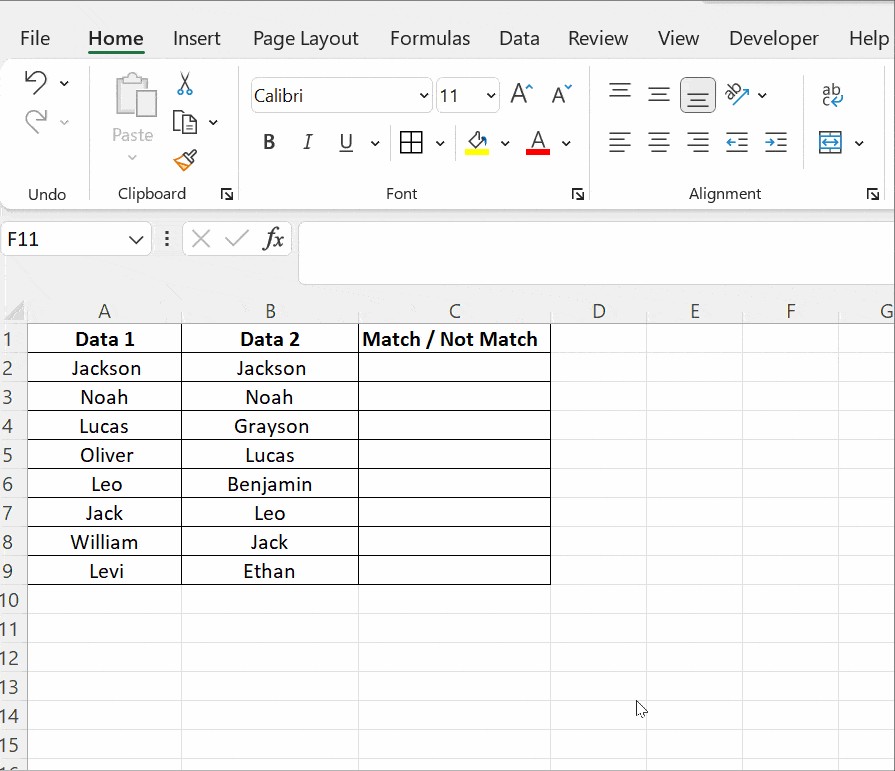
4. Using IF Condition for Enhanced Comparison
The IF condition in Excel allows for more descriptive results, such as “Match” or “Not Match,” instead of simply TRUE or FALSE.
4.1. Identifying Matching Values
To return “Match” for identical values and leave other cells empty, use the formula =IF(A2=B2,”Match”,””).
4.2. Identifying Mismatching Values
To display “Not a Match” for different values, use the formula =IF(A2=B2,”Match”,”Not a Match”).
4.3. Comparing for Differences
To find differences between two columns, replace the equals sign with the non-equality sign (<>): =IF(A2<>B2,”Match”,”Not a Match”).
5. Using the EXACT() Function for Case-Sensitive Comparisons
When comparing text strings, the EXACT() function ensures that the comparison is case-sensitive.
5.1. Syntax and Usage
The syntax for the EXACT() function is =EXACT(text1, text2). It returns TRUE if the text strings are identical, including case, and FALSE otherwise.
5.2. Example
Consider two columns, Data1 and Data2, both containing “Nova Scotia.” Using the formula =IF(A2=B2, “Match”, “Mismatch”) returns “Match” because the comparison is case-insensitive.
However, using =IF(EXACT(A2, B2), “Match”, “Mismatch”) provides a case-sensitive comparison.
5.3. How EXACT() Works
The EXACT() function first evaluates the text strings and then returns TRUE or FALSE to the IF condition. The IF condition then displays the corresponding “Match” or “Mismatch” result.
6. Comparing Two Columns Using Conditional Formatting
Conditional formatting is a powerful tool to highlight duplicate or unique values directly in the columns.
6.1. Highlighting Duplicate Values
- Select the columns you want to compare.
- Go to Home → Styles → Conditional Formatting → Highlight Cells Rules → Duplicate Values.
- Choose “Duplicate” from the drop-down menu and select a formatting style (e.g., fill color, text color).
6.2. Highlighting Unique Values
- Select the columns you want to compare.
- Go to Home → Styles → Conditional Formatting → Highlight Cells Rules → Duplicate Values.
- Choose “Unique” from the drop-down menu and select a formatting style.
6.3. Clearing Conditional Formatting
To remove conditional formatting, go to Conditional Formatting → Clear Rules → Clear Rules from Selected Cells.
6.4. Benefits of Conditional Formatting
Conditional formatting is ideal for smaller tables where a visual representation of matching or unique data is sufficient. It eliminates the need for a third column displaying comparison results.
7. Using Lookup Functions to Compare Two Columns
Lookup functions, such as VLOOKUP, HLOOKUP, and XLOOKUP, are essential for comparing data across different columns or tables.
7.1. VLOOKUP() Function
The VLOOKUP function searches for a value in the first column of a range and returns a value in the same row from another column.
Syntax: =VLOOKUP(lookup_value, table_array, col_index_num, [range_lookup])
- lookup_value: The value to search for.
- table_array: The range in which to search.
- col_index_num: The column number in the range from which to return a value.
- range_lookup: TRUE for approximate match (sorted ascending), FALSE for exact match.
7.2. Example
Suppose column A lists exams taken by a student, and column B lists subjects passed. To determine which subjects were cleared, apply VLOOKUP in cell C2: =VLOOKUP(A2, $B$2:$B$5, 1, 0).
Drag the formula down to apply it to all cells. The result in column C will show the cleared subjects and #N/A for those not cleared.
7.3. Understanding the Formula
- VLOOKUP(A2,..,..,..): Takes the value in cell A2.
- VLOOKUP(A2, $B$2:$B$5,..,..): Compares with values in cells B2 to B5. The absolute reference ($) locks the range.
- VLOOKUP(A2, $B$2:$B$5,1,..): Specifies the column to compare from the lookup value.
- VLOOKUP(A2, $B$2:$B$5,1,0): Uses 0 for an exact match.
8. Comparing Two Columns Using INDEX-MATCH
The INDEX-MATCH function is a flexible alternative to VLOOKUP, especially when matching columns in different tables.
8.1. Syntax
The combination of INDEX and MATCH functions allows for more complex lookups.
- INDEX(array, row_num, [column_num]): Returns the value at a given row and column in a range.
- MATCH(lookup_value, lookup_array, [match_type]): Returns the position of a lookup value in an array.
8.2. Example
To match values from column D with column A and pull corresponding values from column B, use the formula =INDEX($B$2:$B$4, MATCH(D2, $A$2:$A$4, 0)).
This formula searches for the value in D2 within the range A2:A4 and returns the corresponding value from B2:B4.
9. More Ways to Compare Two Columns in Excel
Here’s a deeper dive into additional techniques for comparing two columns in Excel, including advanced conditional formatting, combined formulas, and specialized functions.
9.1. Advanced Conditional Formatting Techniques
Conditional formatting can be used beyond just highlighting duplicates or unique values. It can also be used to apply formatting based on complex criteria derived from comparing two columns.
9.1.1. Using Formulas in Conditional Formatting
You can use formulas to determine which cells to format. This is especially useful when the condition depends on values in other columns.
Example: Suppose you want to highlight cells in column A if their corresponding values in column B are greater than 100.
- Select the range in column A.
- Go to Home → Conditional Formatting → New Rule.
- Select “Use a formula to determine which cells to format”.
- Enter the formula =$B1>100.
- Click Format to choose the formatting style.
- Click OK.
Now, any cell in column A where the corresponding cell in column B is greater than 100 will be highlighted.
9.1.2. Highlighting Entire Rows Based on Column Comparison
Sometimes, you might want to highlight the entire row based on a comparison between two columns.
Example: Highlight the entire row if the values in column A and column B do not match.
- Select the entire data range.
- Go to Home → Conditional Formatting → New Rule.
- Select “Use a formula to determine which cells to format”.
- Enter the formula =$A1<>$B1.
- Click Format to choose the formatting style.
- Click OK.
This will highlight all rows where the values in column A and column B are different.
9.2. Combining Formulas for Complex Comparisons
Excel’s power lies in its ability to combine different formulas to perform complex comparisons. Here are a few examples:
9.2.1. Using IF with AND/OR for Multiple Conditions
You can use the IF function in combination with AND or OR to check multiple conditions at once.
Example: Check if both column A and column B have values greater than 50.
=IF(AND(A1>50, B1>50), “Both > 50”, “Not Both > 50”)
Example: Check if either column A or column B has a value greater than 50.
=IF(OR(A1>50, B1>50), “One > 50”, “Neither > 50”)
9.2.2. Using COUNTIF for Counting Matches
The COUNTIF function can be used to count how many times a value from one column appears in another column.
Example: Count how many times each value in column A appears in column B.
- In cell C1, enter the formula =COUNTIF($B:$B, A1).
- Drag the formula down to apply it to all rows.
Column C will show the number of times each value from column A appears in column B.
9.3. Specialized Functions for Text Comparison
Excel provides specialized functions for more nuanced text comparisons, such as FIND, SEARCH, and SUBSTITUTE.
9.3.1. FIND and SEARCH
The FIND and SEARCH functions are used to find the position of one text string within another. The main difference is that FIND is case-sensitive, while SEARCH is not.
Example: Check if column A contains a specific substring (case-sensitive).
=IF(ISNUMBER(FIND(“substring”, A1)), “Contains”, “Does Not Contain”)
Example: Check if column A contains a specific substring (case-insensitive).
=IF(ISNUMBER(SEARCH(“substring”, A1)), “Contains”, “Does Not Contain”)
9.3.2. SUBSTITUTE
The SUBSTITUTE function replaces a specified text with another text in a string.
Example: Replace all occurrences of “old” with “new” in column A.
=SUBSTITUTE(A1, “old”, “new”)
9.4. Array Formulas for Advanced Comparisons
Array formulas can perform calculations on multiple values at once, making them useful for advanced comparisons.
9.4.1. Comparing Two Columns for Any Differences
To check if there are any differences between two columns, you can use an array formula.
- Select a range of cells where you want the results.
- Enter the formula =SUM(IF(A1:A10<>B1:B10, 1, 0)).
- Press Ctrl + Shift + Enter to enter it as an array formula.
This formula compares each cell in the range A1:A10 with the corresponding cell in B1:B10 and returns the number of differences.
9.4.2. Finding Unique Values Across Two Columns
To find unique values that appear in only one of the two columns, you can use an array formula with COUNTIF.
- Select a range of cells where you want the unique values.
- Enter the formula =IF(COUNTIF(B:B,A1)=0,A1,””) in the first cell.
- Press Ctrl + Shift + Enter to enter it as an array formula.
- Drag the formula down to apply it to all rows.
This formula checks if each value in column A appears in column B. If it doesn’t, it returns the value; otherwise, it returns an empty string.
9.5. Real-World Scenarios
To further illustrate the practical application of these methods, consider the following real-world scenarios:
9.5.1. Data Validation and Cleansing
When importing data from multiple sources, it is common to have inconsistencies. Comparing columns can help you identify and correct these inconsistencies.
Scenario: You have a list of customer names and email addresses from two different databases. Use the EXACT function to identify case-sensitive differences and the SUBSTITUTE function to standardize name formats.
9.5.2. Inventory Management
In inventory management, comparing columns can help you track stock levels, identify discrepancies, and manage orders.
Scenario: Compare a list of products ordered with a list of products received. Use conditional formatting to highlight any discrepancies and the VLOOKUP function to retrieve additional product details from a master product list.
9.5.3. Financial Auditing
Comparing columns is essential in financial auditing to ensure accuracy and compliance.
Scenario: Compare transaction records with bank statements. Use the IF function to identify discrepancies and the SUMIF function to calculate the total value of matching transactions.
10. Frequently Asked Questions
10.1. How do I compare two columns in Excel for differences and highlight the mismatches?
To highlight mismatches, use conditional formatting with the formula =$A1<>$B1. Select your data range, go to Home → Conditional Formatting → New Rule → Use a formula to determine which cells to format, and enter the formula.
10.2. Can I compare two columns in different Excel sheets?
Yes, you can compare columns in different sheets by referencing the sheet name in your formulas. For example, =IF(Sheet1!A1=Sheet2!A1, “Match”, “Mismatch”).
10.3. How can I compare two columns and return a value from a third column if there’s a match?
Use the VLOOKUP or INDEX-MATCH functions. For example, =VLOOKUP(A1, B:C, 2, FALSE) will search for the value in A1 in column B and return the corresponding value from column C if there’s a match.
10.4. What is the best way to compare two columns with thousands of rows?
For large datasets, conditional formatting and formulas can slow down Excel. Using the VLOOKUP or INDEX-MATCH functions is more efficient. Also, ensure your data is well-structured and use Excel’s built-in table features.
10.5. How do I compare two columns and ignore case?
Use the EXACT function for case-sensitive comparisons and the standard equals operator (=) or the SEARCH function for case-insensitive comparisons.
11. Conclusion
Comparing two columns in Excel is a fundamental skill with numerous applications across various fields. Whether you’re using basic formulas, conditional formatting, or advanced functions like VLOOKUP and INDEX-MATCH, understanding these techniques will greatly enhance your data analysis capabilities.
To further enhance your expertise in Excel, explore the comprehensive courses and tutorials available on COMPARE.EDU.VN. Our resources provide in-depth knowledge and practical skills to master Excel functions and formulas, ensuring you can efficiently manage and analyze data.
Ready to take your Excel skills to the next level? Visit COMPARE.EDU.VN today and discover a wealth of resources to help you become an Excel expert. Contact us at:
Address: 333 Comparison Plaza, Choice City, CA 90210, United States
Whatsapp: +1 (626) 555-9090
Website: compare.edu.vn
By mastering these methods, you can streamline your data analysis workflow, make informed decisions, and gain deeper insights from your data. Whether it’s for data validation, inventory management, or financial auditing, the ability to compare columns effectively is an invaluable asset in today’s data-driven world.