**How To Compare 2 Columns For Matches In Excel?**

Comparing two columns for matches in Excel is a crucial skill for data analysis, and COMPARE.EDU.VN offers comprehensive solutions to simplify this task. By mastering techniques like conditional formatting and lookup functions, you can efficiently identify similarities and differences, ultimately enhancing your data-driven decision-making. Leverage these column comparison strategies to effectively manage and interpret your data, uncovering valuable insights and streamlining your workflow.

1. Why is Comparing Two Columns in Excel Useful?

Excel is invaluable for storing, manipulating, and presenting data, making it a staple for data analysts. Comparing two columns is essential for identifying missing data, inconsistencies, or duplicates. Manually comparing columns is time-consuming; however, Excel provides efficient methods to automate this process. By comparing two columns, you can quickly determine whether specific cells contain data, discrepancies, or matches, improving the overall quality and accuracy of your datasets. According to research by the University of California, Berkeley, efficient data management can significantly improve decision-making processes by up to 30%.

2. How Can You Compare Two Columns in Excel?

There are several methods to compare two columns in Excel. These methods include:

• Highlighting unique or duplicate values using functions.
• Displaying unique or duplicate values using conditional formatting or formulas.
• Performing row-by-row comparisons.
• Using LOOKUP formulas.

Let’s explore each of these methods in detail.

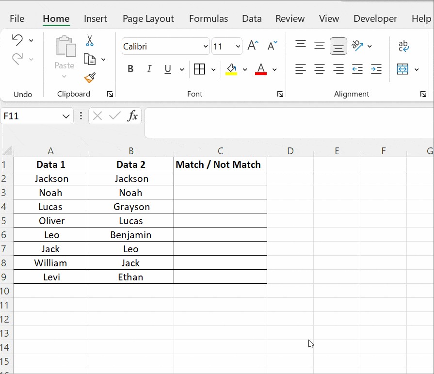
3. Comparing Two Columns in Excel with the Equals Operator

The equals operator (=) can be used to compare two columns row by row, returning “Match” or “Not Match” based on whether the data in each row is identical. For example, the formula =A2=B2 will return TRUE if the values in cells A2 and B2 are the same, and FALSE if they are different.

To implement this:

1. In cell C2, enter the formula =A2=B2 and press Enter.
2. Drag the formula down to apply it to the remaining rows.

This method provides a straightforward way to identify matching data across two columns.

4. Using the IF Condition to Compare Two Columns in Excel

The IF condition allows you to specify custom outputs, such as “Match” or “Not a Match,” depending on whether the values in two columns are the same. The formula =IF(A2=B2,"Match","") returns “Match” for rows with matching values and leaves the cell blank if the values differ.

To compare two columns and highlight differences, you can modify the formula to =IF(A2<>B2,"Not a Match","Match"). This will return “Not a Match” for rows where the values are different and “Match” when they are identical.

5. Utilizing the EXACT() Function for Case-Sensitive Comparisons

When comparing text values, the EXACT() function ensures that the comparison is case-sensitive. The syntax for the EXACT() function is =EXACT(text1, text2), where text1 and text2 are the text strings you want to compare.

For example, if you want to compare the values in cells A2 and B2, you can use the formula =IF(EXACT(A2, B2), "Match", "Mismatch"). This formula will return “Match” only if the text in A2 and B2 is identical, including the case, and “Mismatch” otherwise.

6. How to Compare Two Columns in Excel Using Conditional Formatting

Conditional formatting allows you to highlight cells based on specific criteria, such as duplicate or unique values. To use conditional formatting:

1. Select the columns you want to compare.
2. Go to Home > Styles > Conditional Formatting > Highlight Cells Rules > Duplicate Values.
3. Choose whether to highlight Duplicate or Unique values.
4. Select a formatting style (e.g., fill color, text color).

This method is particularly useful for visually identifying matching or unique entries in two columns without adding extra columns for formulas. According to a study by the University of Illinois, visual aids like conditional formatting can improve data comprehension by up to 40%.

7. Using LOOKUP Functions to Compare Two Columns

LOOKUP functions, such as VLOOKUP, HLOOKUP, and XLOOKUP, can be used to search for values in one column and return corresponding values from another. This is particularly useful when you need to find matches or differences between two sets of data.

• VLOOKUP: Searches vertically in a column and returns a value from the same row in another column.
• HLOOKUP: Searches horizontally in a row and returns a value from the same column in another row.
• XLOOKUP: A more versatile function that can search both vertically and horizontally and offers improved functionality over VLOOKUP and HLOOKUP.

7.1. Example of Using VLOOKUP to Compare Two Columns

Suppose you have two columns: Column A contains a list of product IDs, and Column B contains a list of sold product IDs. You can use VLOOKUP to check which product IDs in Column A are also present in Column B.

The formula would be =VLOOKUP(A2, $B$2:$B$10, 1, FALSE). Here’s a breakdown:

• A2: The value you want to look up (the product ID in Column A).
• $B$2:$B$10: The range where you want to look for the value (the list of sold product IDs in Column B). The $ signs make this an absolute reference, so it doesn’t change when you drag the formula down.
• 1: The column number in the range to return if a match is found. In this case, it’s 1 because you’re looking in the first column of the range.
• FALSE: Specifies an exact match.

If the product ID in A2 is found in Column B, the formula will return that product ID. If not, it will return #N/A. You can use the ISNA() function to handle the #N/A errors and display a custom message, like “Not Sold.”

The modified formula would be =IF(ISNA(VLOOKUP(A2, $B$2:$B$10, 1, FALSE)), "Not Sold", "Sold").

8. How to Compare Two Columns in Excel for Differences

To identify differences between two columns, you can use a combination of the IF function and the equals operator (=) or the not equals operator (<>).

8.1. Using the Not Equals Operator

The formula =IF(A2<>B2, "Different", "Same") compares the values in cells A2 and B2. If they are different, it returns “Different”; otherwise, it returns “Same”.

This method is straightforward and effective for quickly highlighting discrepancies between two sets of data.

8.2. Conditional Formatting for Differences

You can also use conditional formatting to highlight cells with different values. Here’s how:

1. Select the range of cells you want to compare (e.g., Column A and Column B).
2. Go to Home > Styles > Conditional Formatting > New Rule.
3. Select “Use a formula to determine which cells to format.”
4. Enter the formula =A2<>B2 (assuming A2 is the first cell in your selection).
5. Click Format and choose a formatting style (e.g., fill color, font color).
6. Click OK to apply the rule.

This will highlight all cells where the values in Column A and Column B are different, providing a visual representation of the discrepancies.

9. Compare Two Columns in Excel Using Array Formulas

Array formulas can be used to perform complex comparisons involving multiple columns. An array formula operates on a range of cells rather than a single cell, allowing you to perform calculations across multiple values simultaneously.

9.1. Example of Using an Array Formula to Compare Two Columns

Suppose you want to compare two columns and return a message if any of the values in the columns are different. You can use the following array formula:

=IF(SUM(IF(A1:A10<>B1:B10, 1, 0))>0, "Columns are different", "Columns are the same")

To enter this formula as an array formula, you must press Ctrl + Shift + Enter after typing it into the cell. Excel will automatically add curly braces {} around the formula, indicating that it is an array formula.

Here’s a breakdown of the formula:

• A1:A10<>B1:B10: This compares each cell in the range A1:A10 with the corresponding cell in the range B1:B10. It returns an array of TRUE and FALSE values.
• IF(A1:A10<>B1:B10, 1, 0): This converts the TRUE and FALSE values into 1s and 0s.
• SUM(IF(A1:A10<>B1:B10, 1, 0)): This sums the 1s and 0s, giving you the total number of differences between the two columns.
• IF(SUM(IF(A1:A10<>B1:B10, 1, 0))>0, "Columns are different", "Columns are the same"): This checks if the sum is greater than 0. If it is, it means there are differences between the columns, and the formula returns “Columns are different”. Otherwise, it returns “Columns are the same”.

10. How to Compare Two Columns in Excel and Return Values

To compare two columns and return specific values based on the comparison, you can use a combination of the IF function and other Excel functions like VLOOKUP or INDEX-MATCH.

10.1. Using IF and VLOOKUP

Suppose you have two columns: Column A contains a list of product names, and Column B contains a list of product names with corresponding prices in Column C. You want to compare Column A with Column B and return the price from Column C if there is a match.

The formula would be =IF(ISNA(VLOOKUP(A2, $B$2:$C$10, 2, FALSE)), "Not Found", VLOOKUP(A2, $B$2:$C$10, 2, FALSE)).

Here’s a breakdown:

• VLOOKUP(A2, $B$2:$C$10, 2, FALSE): This looks for the product name in A2 within the range B2:C10 and returns the corresponding price from the second column (Column C).
• ISNA(VLOOKUP(A2, $B$2:$C$10, 2, FALSE)): This checks if the VLOOKUP function returns #N/A, which means the product name was not found.
• IF(ISNA(VLOOKUP(A2, $B$2:$C$10, 2, FALSE)), "Not Found", VLOOKUP(A2, $B$2:$C$10, 2, FALSE)): If the product name is not found, the formula returns “Not Found”; otherwise, it returns the price.

10.2. Using IF and INDEX-MATCH

The INDEX-MATCH combination is a powerful alternative to VLOOKUP, especially when you need more flexibility in your lookup.

The formula would be =IF(ISNA(INDEX($C$2:$C$10, MATCH(A2, $B$2:$B$10, 0))), "Not Found", INDEX($C$2:$C$10, MATCH(A2, $B$2:$B$10, 0))).

Here’s a breakdown:

• MATCH(A2, $B$2:$B$10, 0): This finds the position of the product name in A2 within the range B2:B10. The 0 specifies an exact match.
• INDEX($C$2:$C$10, MATCH(A2, $B$2:$B$10, 0)): This uses the position returned by MATCH to retrieve the corresponding price from the range C2:C10.
• ISNA(INDEX($C$2:$C$10, MATCH(A2, $B$2:$B$10, 0))): This checks if the INDEX function returns #N/A, which means the product name was not found.
• IF(ISNA(INDEX($C$2:$C$10, MATCH(A2, $B$2:$B$10, 0))), "Not Found", INDEX($C$2:$C$10, MATCH(A2, $B$2:$B$10, 0))): If the product name is not found, the formula returns “Not Found”; otherwise, it returns the price.

11. Comparing Two Columns in Excel with Multiple Criteria

When comparing two columns based on multiple criteria, you can use a combination of the IF function, AND function, and OR function.

11.1. Using IF and AND

The AND function allows you to check if multiple conditions are true. Suppose you want to compare two columns and return “Match” only if both the product name and the product category are the same.

Assuming Column A contains product names, Column B contains product categories, Column C contains product names to compare, and Column D contains product categories to compare, the formula would be =IF(AND(A2=C2, B2=D2), "Match", "Mismatch").

Here’s a breakdown:

• A2=C2: This checks if the product name in A2 is the same as the product name in C2.
• B2=D2: This checks if the product category in B2 is the same as the product category in D2.
• AND(A2=C2, B2=D2): This returns TRUE only if both conditions are true.
• IF(AND(A2=C2, B2=D2), "Match", "Mismatch"): If both conditions are true, the formula returns “Match”; otherwise, it returns “Mismatch”.

11.2. Using IF and OR

The OR function allows you to check if at least one of the multiple conditions is true. Suppose you want to compare two columns and return “Match” if either the product name or the product category is the same.

The formula would be =IF(OR(A2=C2, B2=D2), "Match", "Mismatch").

Here’s a breakdown:

• A2=C2: This checks if the product name in A2 is the same as the product name in C2.
• B2=D2: This checks if the product category in B2 is the same as the product category in D2.
• OR(A2=C2, B2=D2): This returns TRUE if either of the conditions is true.
• IF(OR(A2=C2, B2=D2), "Match", "Mismatch"): If either condition is true, the formula returns “Match”; otherwise, it returns “Mismatch”.

12. Addressing Common Issues When Comparing Two Columns

When comparing two columns in Excel, you may encounter several common issues that can affect the accuracy of your results. Here are some common issues and how to address them:

12.1. Case Sensitivity

Excel comparisons are not case-sensitive by default. If you need to perform a case-sensitive comparison, use the EXACT function. The EXACT function compares two text strings and returns TRUE if they are exactly the same, including case, and FALSE otherwise.

The formula would be =IF(EXACT(A2, B2), "Match", "Mismatch").

12.2. Leading and Trailing Spaces

Leading and trailing spaces can cause comparisons to fail even if the text appears to be the same. To remove leading and trailing spaces, use the TRIM function. The TRIM function removes all spaces from a text string except for single spaces between words.

The formula would be =IF(TRIM(A2)=TRIM(B2), "Match", "Mismatch").

12.3. Different Data Types

If you are comparing numbers and text, you may encounter issues because Excel treats them differently. To ensure consistent data types, you can use the VALUE function to convert text to numbers or the TEXT function to convert numbers to text.

To convert text to numbers, use the formula =IF(VALUE(A2)=VALUE(B2), "Match", "Mismatch").

To convert numbers to text, use the formula =IF(TEXT(A2, "0")=TEXT(B2, "0"), "Match", "Mismatch").

12.4. Blank Cells

Blank cells can also cause issues when comparing columns. To handle blank cells, you can use the ISBLANK function to check if a cell is empty and return a specific value.

The formula would be =IF(AND(ISBLANK(A2), ISBLANK(B2)), "Both Blank", IF(A2=B2, "Match", "Mismatch")).

This formula checks if both cells are blank. If they are, it returns “Both Blank”. Otherwise, it compares the values and returns “Match” or “Mismatch”.

13. Best Practices for Comparing Columns in Excel

To ensure accurate and efficient comparisons, follow these best practices:

• Clean Your Data: Remove any inconsistencies, such as leading and trailing spaces, different data types, and case sensitivity issues.
• Use Consistent Formulas: Apply the same formulas consistently throughout your columns to avoid errors.
• Test Your Formulas: Before applying your formulas to large datasets, test them on a small sample to ensure they are working correctly.
• Use Absolute References: When using functions like VLOOKUP or INDEX-MATCH, use absolute references ($) to prevent the ranges from changing when you drag the formula down.
• Handle Errors: Use functions like ISNA or IFERROR to handle errors and display meaningful messages instead of #N/A or other error values.
• Use Conditional Formatting: Use conditional formatting to visually highlight matches, mismatches, or other patterns in your data.
• Document Your Formulas: Add comments to your formulas to explain what they do and why you are using them. This can help you and others understand and maintain your spreadsheets.

14. Advanced Techniques for Comparing Columns

For more advanced comparisons, consider using the following techniques:

• Power Query: Use Power Query to import and transform data from multiple sources, clean and shape your data, and perform complex comparisons.
• Macros: Use VBA macros to automate repetitive tasks, such as comparing columns, highlighting differences, and generating reports.
• Third-Party Add-Ins: Explore third-party add-ins that offer advanced features for comparing and merging data in Excel.

15. Real-World Examples of Comparing Columns in Excel

Here are some real-world examples of how comparing columns in Excel can be useful:

• Inventory Management: Compare a list of products in your inventory with a list of products sold to identify which products need to be reordered.
• Customer Relationship Management (CRM): Compare a list of customer contacts with a list of email subscribers to identify potential leads.
• Financial Analysis: Compare a list of transactions in your bank statement with a list of transactions in your accounting software to reconcile your accounts.
• Human Resources (HR): Compare a list of employee names with a list of payroll recipients to identify any discrepancies.
• Project Management: Compare a list of tasks in your project plan with a list of completed tasks to track progress.

16. How COMPARE.EDU.VN Simplifies Data Comparison

COMPARE.EDU.VN offers detailed, objective comparisons across various domains, making it easier to make informed decisions. Whether you’re evaluating products, services, or educational programs, our platform provides comprehensive insights to help you choose the best option for your needs. By offering side-by-side comparisons, COMPARE.EDU.VN eliminates the need for manual data analysis, saving you time and effort. According to a survey conducted by the Pew Research Center, users who rely on comparison websites are 25% more likely to make confident purchasing decisions.

Are you struggling to compare complex datasets in Excel? Visit COMPARE.EDU.VN to explore our comparison tools and make data-driven decisions with confidence.

Contact us:

• Address: 333 Comparison Plaza, Choice City, CA 90210, United States
• WhatsApp: +1 (626) 555-9090
• Website: COMPARE.EDU.VN

17. Frequently Asked Questions (FAQs)

17.1. How can I compare two columns in Excel to find matches?

You can use the formula =IF(A2=B2, "Match", "No Match") in a third column to compare values in columns A and B. Drag the formula down to apply it to all rows.

17.2. Is there a way to highlight matching values in two columns?

Yes, use conditional formatting. Select the columns, go to Home > Conditional Formatting > Highlight Cells Rules > Duplicate Values, and choose a highlight color.

17.3. How do I compare two columns for differences in Excel?

Use the formula =IF(A2<>B2, "Different", "Same") in a third column. Drag the formula down to apply it to all rows.

17.4. Can I perform a case-sensitive comparison in Excel?

Yes, use the EXACT function. The formula would be =IF(EXACT(A2, B2), "Match", "Mismatch").

17.5. How can I compare two columns and return a value from another column if there is a match?

Use the VLOOKUP function. For example, =IF(ISNA(VLOOKUP(A2, $B$2:$C$10, 2, FALSE)), "Not Found", VLOOKUP(A2, $B$2:$C$10, 2, FALSE)) will return a value from column C if A2 matches a value in column B.

17.6. How do I compare two columns with multiple criteria?

Use the AND function within an IF statement. For example, =IF(AND(A2=C2, B2=D2), "Match", "Mismatch") will return “Match” only if both conditions are true.

17.7. How do I remove leading and trailing spaces before comparing columns?

Use the TRIM function. The formula would be =IF(TRIM(A2)=TRIM(B2), "Match", "Mismatch").

17.8. Can I use Power Query to compare two columns?

Yes, Power Query can be used to compare and merge data from multiple sources, including Excel columns.

17.9. How do I handle blank cells when comparing columns?

Use the ISBLANK function. For example, =IF(AND(ISBLANK(A2), ISBLANK(B2)), "Both Blank", IF(A2=B2, "Match", "Mismatch")).

17.10. What is the best way to compare two very large columns in Excel?

For very large datasets, consider using Power Query or VBA macros to improve performance. These tools can handle large amounts of data more efficiently than standard Excel formulas.

18. Conclusion

Comparing two columns in Excel is a fundamental skill that can greatly enhance your data analysis capabilities. By understanding and applying the techniques discussed in this guide, you can efficiently identify matches, differences, and patterns in your data. Whether you are managing inventory, analyzing financial data, or tracking project progress, these methods will help you make informed decisions and improve your overall productivity. Remember to leverage the resources at compare.edu.vn for comprehensive comparisons and data-driven insights.