How To Compare 2 Columns In Excel: A Comprehensive Guide?

Comparing two columns in Excel is essential for data analysis, verification, and cleaning, and COMPARE.EDU.VN offers comprehensive resources to master this skill. This guide provides various methods to identify matches, discrepancies, and unique values efficiently. Discover techniques to streamline your spreadsheet tasks and ensure data accuracy for informed decision-making, enhancing data integrity, and achieving efficient data comparison.

1. Understanding the Basics of Column Comparison in Excel

Comparing columns in Excel involves checking cells against each other to identify matches, differences, or unique entries. This process is crucial for tasks ranging from verifying data accuracy to identifying discrepancies in large datasets. Mastering column comparison techniques can significantly improve data management and analysis skills. Whether you’re working with financial records, customer lists, or scientific data, knowing how to effectively compare columns in Excel will help you make informed decisions and maintain data integrity, all while leveraging effective data matching.

2. Utilizing Conditional Formatting for Quick Comparisons

Conditional formatting is a straightforward method for comparing columns in Excel, allowing you to highlight duplicate or unique values quickly.

2.1. Highlighting Duplicate Values

To highlight duplicate values, follow these steps:

Select the Range: Select the columns you want to compare.
Access Conditional Formatting: Go to the “Home” tab, click on “Conditional Formatting,” then “Highlight Cells Rules,” and select “Duplicate Values.”
Choose Formatting: Choose the formatting style (e.g., fill color) to highlight duplicate values.

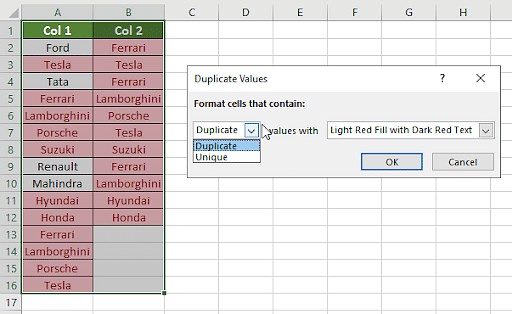
2.2. Identifying Unique Values

To identify unique values:

Select the Range: Select the columns you want to compare.
Access Conditional Formatting: Go to the “Home” tab, click on “Conditional Formatting,” then “Highlight Cells Rules,” and select “Duplicate Values.”
Select Unique: In the dialog box, choose “Unique” instead of “Duplicate.”
Choose Formatting: Select the desired formatting style to highlight unique values.

2.3. Advantages of Conditional Formatting

Quick Identification: Instantly highlights matches or differences.
Visual Aid: Provides a clear visual representation of data discrepancies.
Easy to Apply: Simple steps make it accessible for users of all skill levels.

3. Employing the Equals Operator for Direct Comparison

The equals operator (=) provides a direct way to compare corresponding cells in two columns, displaying TRUE for matches and FALSE for differences.

3.1. Basic Implementation

Create a Result Column: Insert a new column next to the columns you want to compare.
Enter the Formula: In the first cell of the new column, enter the formula =A1=B1 (assuming the first data cell in column A is A1 and in column B is B1).
Apply to All Cells: Drag the fill handle (the small square at the bottom-right of the cell) down to apply the formula to all rows.

3.2. Customizing Results with the IF Function

To display custom messages instead of TRUE or FALSE:

Modify the Formula: Use the IF function to display specific text. For example, =IF(A1=B1, "Match", "Mismatch").
Apply to All Cells: Drag the fill handle down to apply the formula to all rows.

3.3. Advantages of the Equals Operator

Simple and Direct: Easy to understand and implement.
Customizable: Can be combined with the IF function for more informative results.
Real-Time Comparison: Results update automatically if the source data changes.

4. Leveraging the VLOOKUP Function for Detailed Analysis

VLOOKUP is a powerful function for finding values in one column based on matches in another column. It’s particularly useful for comparing lists and identifying missing entries.

4.1. Basic VLOOKUP Formula

The VLOOKUP formula is structured as follows:

=VLOOKUP(lookup_value, table_array, col_index_num, [range_lookup])

lookup_value: The value to search for in the first column of the table.
table_array: The range of cells containing the data to search.
col_index_num: The column number in the table_array from which to return a value.
[range_lookup]: TRUE for an approximate match, FALSE for an exact match.

4.2. Comparing Columns with VLOOKUP

Create a Result Column: Insert a new column where you want the comparison results.
Enter the Formula: In the first cell of the new column, enter the VLOOKUP formula. For example, if you want to check if values in column A exist in column B, use =VLOOKUP(A1, B:B, 1, FALSE).
Handle Errors: Use the IFERROR function to display a custom message when a match is not found. For example, =IFERROR(VLOOKUP(A1, B:B, 1, FALSE), "Not Found").
Apply to All Cells: Drag the fill handle down to apply the formula to all rows.

4.3. Addressing Partial Matches with Wildcards

In cases where you need to compare data with slight variations, such as “Ford India” vs. “Ford,” you can use wildcards:

Modify the Formula: Add a wildcard to the lookup_value. For example, =IFERROR(VLOOKUP(A1&"*", B:B, 1, FALSE), "Not Found").

4.4. Advantages of VLOOKUP

Versatile: Can find exact or approximate matches.
Informative: Returns values from corresponding rows, providing additional context.
Error Handling: IFERROR function allows for graceful handling of missing values.

5. Applying the IF Formula for Conditional Results

The IF formula is used to compare 2 columns in Excel when you want to display a desired result for a similarity or a difference.

5.1. Basic IF Formula

The IF formula is structured as follows:

=IF(condition, value_if_true, value_if_false)

condition: The condition to test.
value_if_true: The value to return if the condition is TRUE.
value_if_false: The value to return if the condition is FALSE.

5.2. Comparing Columns with IF

Create a Result Column: Insert a new column where you want the comparison results.
Enter the Formula: In the first cell of the new column, enter the IF formula. For example, if you want to check if values in column A are equal to values in column B, use =IF(A1=B1, "Match", "Mismatch").
Apply to All Cells: Drag the fill handle down to apply the formula to all rows.

5.3. Advantages of IF Formula

Simple and Direct: Easy to understand and implement.
Customizable: Allows for custom messages based on the comparison result.
Clear Results: Provides a straightforward way to identify matches and mismatches.

6. Utilizing the EXACT Formula for Case-Sensitive Comparisons

The EXACT formula is used to compare two columns in Excel, taking into account the case of the text.

6.1. Basic EXACT Formula

The EXACT formula is structured as follows:

=EXACT(text1, text2)

text1: The first text string.
text2: The second text string.

6.2. Comparing Columns with EXACT

Create a Result Column: Insert a new column where you want the comparison results.
Enter the Formula: In the first cell of the new column, enter the EXACT formula. For example, if you want to check if values in column A are exactly equal to values in column B, use =EXACT(A1,B1).
Apply to All Cells: Drag the fill handle down to apply the formula to all rows.

6.3. Advantages of EXACT Formula

Case-Sensitive: Distinguishes between uppercase and lowercase letters.
Precise Comparison: Ensures that the compared values are identical.
Clear Results: Provides a straightforward way to identify exact matches and mismatches.

7. Choosing the Right Comparison Method for Different Scenarios

Selecting the appropriate method depends on the specific requirements of your comparison task. Here’s a guide to help you choose:

7.1. Comparing Two Columns Row-by-Row

For simple row-by-row comparisons, use the equals operator (=) or the IF function.

Formulas:
- =IF(A2=B2, "Match", " ")
- =IF(A2<>B2, "No Match", " ")
- =IF(A2=B2, "Match", "No Match")

For case-sensitive comparisons, use the EXACT function:

Formulas:
- =IF(EXACT(A2, B2), "Match", " ")
- =IF(EXACT(A2, B2), "Match", "No Match")

7.2. Comparing Multiple Columns for Row Matches

To compare more than two columns, use the AND or COUNTIF functions.

Formulas:
- =IF(AND(A2=B2, A2=C2), "Complete Match", " ")
- =IF(COUNTIF($A2:$E2, $A2)=4, "Complete Match", " ") (where 4 is the number of columns being compared)

To compare columns and identify if any two or more cells have the same values, use the OR function:

Formulas:
- =IF(OR(A2=B2, B2=C2, A2=C2), "Match", "")
- =IF(COUNTIF(B2:D2, A2)+COUNTIF(C2:D2, B2)+(C2=D2)=0, "Unique", "Match")

7.3. Comparing Two Columns for Matches and Differences

To find unique values in column A that are not present in column B, use the COUNTIF or MATCH functions:

Formulas:
- =IF(COUNTIF($B:$B, $A2)=0, "Not Present in B", "")
- =IF(ISERROR(MATCH($A2, $B$2:$B$10, 0)), "Not Present in B", "")

To get results for both matches and unique values:

Formula:
- =IF(COUNTIF($B:$B, $A2)=0, "Not Present in B", "Present in B")

7.4. Comparing Two Lists and Pulling Matching Data

Use VLOOKUP, INDEX MATCH, or XLOOKUP to compare two lists and retrieve matching data:

Formulas:
- =VLOOKUP(D2, $A$2:$B$6, 2, FALSE)
- =INDEX($B$2:$B$6, MATCH($D2, $A$2:$A$6, 0))
- =XLOOKUP(D2, $A$2:$A$6, $B$2:$B$6)

7.5. Highlighting Row Matches and Differences

Use conditional formatting to highlight rows with identical values in all columns:

Formula:
- =AND($A2=$B2, $A2=$C2)
- =COUNTIF($A2:$C2, $A2)=3 (where 3 is the number of columns)

Alternatively, follow these steps:

Select Columns: Select the columns to compare.
Go To Special: Go to the “Home” tab, click “Find & Select,” and choose “Go To Special.”
Select Row Differences: Select “Row Differences” and click “OK.”
Format: The cells with different values will be highlighted.

8. Advanced Techniques for Complex Comparisons

For more complex scenarios, consider using advanced formulas and techniques:

8.1. Using Array Formulas

Array formulas allow you to perform calculations on multiple values at once. For example, to compare two columns and return an array of TRUE/FALSE values:

Select a Range: Select a range of cells where you want the results.
Enter the Formula: Enter the formula =A1:A10=B1:B10 and press Ctrl + Shift + Enter.

8.2. Combining Functions

Combine multiple functions to create more sophisticated comparisons. For example, to check if a value in column A exists in column B and return a corresponding value from column C:

Formula:
- =IFERROR(INDEX(C:C, MATCH(A1, B:B, 0)), "Not Found")

8.3. Using Power Query

Power Query is a powerful data transformation and analysis tool within Excel. You can use it to compare and merge data from multiple sources, identify differences, and perform complex data manipulations.

9. Best Practices for Efficient Column Comparison

Use Consistent Data Types: Ensure that the data types in the columns being compared are consistent (e.g., text, numbers, dates).
Clean Your Data: Remove any leading or trailing spaces, and correct any inconsistencies in spelling or formatting.
Use Absolute References: When using formulas, use absolute references ($) to prevent cell references from changing when you copy the formula.
Test Your Formulas: Always test your formulas on a small sample of data before applying them to the entire dataset.
Document Your Work: Keep a record of the methods and formulas you use, so you can easily replicate your analysis in the future.

10. Real-World Applications of Column Comparison

Column comparison techniques are applicable in various real-world scenarios:

Data Validation: Verifying the accuracy and consistency of data entered into a spreadsheet.
List Management: Identifying duplicate or missing entries in lists of customers, products, or contacts.
Financial Analysis: Comparing financial statements, identifying discrepancies, and tracking changes over time.
Inventory Management: Comparing inventory records, identifying discrepancies, and tracking stock levels.
Scientific Research: Comparing experimental data, identifying patterns, and verifying results.

11. Conclusion: Mastering Column Comparison in Excel

Comparing columns in Excel is a fundamental skill for data analysis and management. By mastering the techniques outlined in this guide, you can efficiently identify matches, differences, and unique values, ensuring data accuracy and enabling informed decision-making. Whether you’re using conditional formatting for quick visual comparisons, the equals operator for direct checks, or VLOOKUP for detailed analysis, these methods will streamline your spreadsheet tasks and enhance your productivity. For more in-depth tutorials and resources, visit COMPARE.EDU.VN, where you can find a wealth of information to help you excel in data analysis.

Facing challenges comparing data and making informed decisions? Visit COMPARE.EDU.VN for comprehensive comparisons and expert insights to simplify your choices.

Address: 333 Comparison Plaza, Choice City, CA 90210, United States
Whatsapp: +1 (626) 555-9090
Website: compare.edu.vn

12. Frequently Asked Questions (FAQs)

12.1. How do I compare two columns in Excel?

Select both columns of data, go to the Home tab, click on Find & Select, choose Go To Special, select Row Differences, and click OK.

12.2. Can I compare two columns in Excel using the Index-Match function?

Yes, you can compare two columns in Excel using the Index-Match function by creating the required formula for the data needed.

12.3. How do I compare multiple columns in Excel?

To compare multiple columns in Excel, you can use the conditional formatting option on the Home tab and format the setting to “duplicates” or “uniques,” and choose the desired color to highlight the values.

12.4. How do you compare two lists in Excel for matches?

You can compare two lists in Excel using IF function, MATCH function, or highlighting row differences.

12.5. How can I compare columns and highlight the first occurrence of a mismatch?

Use Conditional Formatting with a formula like =A1<>B1 to highlight cells where the values differ.

12.6. How do I compare columns for duplicates only?

Use the formula =COUNTIF(B:B, A1)>0 to find duplicates between columns A and B.

12.7. Can I compare columns and count the number of matches or differences?

Yes, use formulas like =SUMPRODUCT(–(A1:A10=B1:B10)) to count matches or =COUNTIF(A1:A10, “B1:B10”) for differences.

12.8. Is there a way to ignore case when comparing columns in Excel?

Yes, use the UPPER or LOWER functions to convert both columns to the same case before comparing. For example, =IF(UPPER(A1)=UPPER(B1), "Match", "Mismatch").

12.9. How can I compare two columns and return a value from a third column if there is a match?

Use the VLOOKUP or INDEX-MATCH functions. For example, =IFERROR(INDEX(C:C, MATCH(A1, B:B, 0)), "Not Found") will return the value from column C if A1 is found in column B.

12.10. What is the best way to compare two columns for partial matches?

Use wildcards with the VLOOKUP function or combine functions like SEARCH and IF. For example, =IF(ISNUMBER(SEARCH(A1, B1)), "Partial Match", "No Match").