Comparing two columns of data in Excel can be a game-changer for data analysis, discrepancy identification, and report cleaning. This comprehensive guide on How To Compare 2 Columns Data In Excel will walk you through various methods to achieve this, from simple formulas to Excel’s built-in tools, ensuring you can identify differences and similarities quickly and efficiently. Let’s get started with how to compare 2 columns data in excel, and for more advanced data comparison techniques, visit COMPARE.EDU.VN.
1. Understanding Column Comparison in Excel
Column comparison in Excel involves checking corresponding cells in two columns to identify matches and discrepancies. This can be crucial for data validation, tracking changes, and ensuring data integrity. Mastering how to compare 2 columns data in excel provides a robust foundation for efficient data management.
1.1. Why Compare Columns in Excel?
Comparing columns in Excel is essential for various reasons:
- Data Validation: Verify data consistency and accuracy between different sources.
- Change Tracking: Identify updates or modifications made to datasets over time.
- Data Cleaning: Locate and correct errors or inconsistencies in your data.
- Report Generation: Ensure the accuracy of reports by comparing data across different tables.
- Auditing: Detect discrepancies and anomalies in financial or operational data.
1.2. Common Scenarios for Column Comparison
Understanding how to compare 2 columns data in excel is useful in numerous scenarios, including:
- Inventory Management: Comparing current stock levels with sales records to identify discrepancies.
- Customer Database Management: Ensuring customer information is consistent across multiple databases.
- Financial Analysis: Comparing budget figures with actual expenditures to identify variances.
- Sales Tracking: Monitoring sales performance by comparing current sales data with previous periods.
- Project Management: Tracking project milestones by comparing planned dates with actual completion dates.
2. Methods to Compare Two Columns in Excel
Several methods can be employed to compare two columns in Excel, each offering unique advantages depending on your specific needs. Here’s a detailed look at each method:
2.1. Conditional Formatting
Conditional formatting is a quick and easy way to highlight differences or matches between two columns.
2.1.1. Highlighting Duplicate Values
Conditional formatting can be used to highlight duplicate values between two columns, allowing you to quickly identify matching data.
Step 1: Select the Data Range
Select all the cells in the two columns you want to compare.
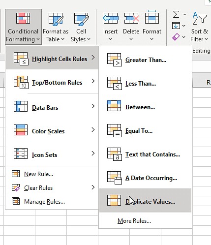
Step 2: Access Conditional Formatting
Go to the “Home” tab on the Excel ribbon and click on “Conditional Formatting” in the “Styles” group.
Step 3: Highlight Duplicate Values
Select “Highlight Cells Rules” and then “Duplicate Values.”
Step 4: Choose Formatting Options
In the “Duplicate Values” dialog box, you can choose the formatting style you want to apply to the duplicate values (e.g., fill color, font color). Click “OK” to apply the formatting.
2.1.2. Highlighting Unique Values
You can also use conditional formatting to highlight unique values, identifying data entries that are present in one column but not the other.
Step 1: Select the Data Range
Select all the cells in the two columns you want to compare.
Step 2: Access Conditional Formatting
Go to the “Home” tab and click on “Conditional Formatting.”
Step 3: Highlight Unique Values
Select “Highlight Cells Rules” and then “Unique Values.”
Step 4: Choose Formatting Options
In the “Unique Values” dialog box, select the desired formatting style for unique values and click “OK.”
2.2. Using the Equals Operator (=)
The equals operator is a simple yet effective way to compare corresponding cells in two columns.
Step 1: Create a Result Column
Insert a new column next to the columns you want to compare.
Step 2: Enter the Formula
In the first cell of the result column, enter the formula =A2=B2 (assuming your data starts in row 2 and you are comparing columns A and B).
Step 3: Apply the Formula to All Cells
Drag the fill handle (the small square at the bottom-right of the cell) down to apply the formula to all the rows you want to compare.
Step 4: Interpret the Results
The result column will display “TRUE” if the values in the corresponding cells are equal and “FALSE” if they are not.
2.3. Using the IF Formula
The IF formula allows you to display custom messages based on whether the values in two cells match.
Step 1: Create a Result Column
Insert a new column next to the columns you want to compare.
Step 2: Enter the Formula
In the first cell of the result column, enter the formula =IF(A2=B2, "Match", "Mismatch").
Step 3: Apply the Formula to All Cells
Drag the fill handle down to apply the formula to all the rows.
Step 4: Interpret the Results
The result column will display “Match” if the values in the corresponding cells are equal and “Mismatch” if they are not.
2.4. Using the VLOOKUP Function
The VLOOKUP function is useful for finding matches between two columns, especially when one column contains a master list.
Step 1: Create a Result Column
Insert a new column next to the column you want to search for matches in.
Step 2: Enter the Formula
In the first cell of the result column, enter the formula =VLOOKUP(A2,B:B,1,FALSE) (assuming you are looking for matches from column A in column B).
Step 3: Handle Errors
To avoid errors when a value is not found, use the IFERROR function: =IFERROR(VLOOKUP(A2,B:B,1,FALSE), "Not Found").
Step 4: Apply the Formula to All Cells
Drag the fill handle down to apply the formula to all the rows.
Step 5: Interpret the Results
The result column will display the matching value from column B if found, or “Not Found” if the value from column A is not present in column B.
2.5. Using the EXACT Function
The EXACT function is case-sensitive and compares two strings to see if they are exactly the same.
Step 1: Create a Result Column
Insert a new column next to the columns you want to compare.
Step 2: Enter the Formula
In the first cell of the result column, enter the formula =EXACT(A2,B2).
Step 3: Apply the Formula to All Cells
Drag the fill handle down to apply the formula to all the rows.
Step 4: Interpret the Results
The result column will display “TRUE” if the values in the corresponding cells are exactly the same (including case) and “FALSE” if they are not.
3. Advanced Techniques for Column Comparison
For more complex scenarios, you can use advanced techniques to compare columns in Excel.
3.1. Comparing Multiple Columns
When you need to compare more than two columns, you can combine formulas to achieve the desired result.
3.1.1. Using the AND Function
The AND function can be used to check if multiple conditions are true.
Step 1: Create a Result Column
Insert a new column next to the columns you want to compare.
Step 2: Enter the Formula
In the first cell of the result column, enter the formula =IF(AND(A2=B2, A2=C2), "Match", "Mismatch") (assuming you are comparing columns A, B, and C).
Step 3: Apply the Formula to All Cells
Drag the fill handle down to apply the formula to all the rows.
Step 4: Interpret the Results
The result column will display “Match” if the values in all corresponding cells are equal and “Mismatch” if they are not.
3.1.2. Using the COUNTIF Function
The COUNTIF function can be used to count the number of times a value appears in a range.
Step 1: Create a Result Column
Insert a new column next to the columns you want to compare.
Step 2: Enter the Formula
In the first cell of the result column, enter the formula =IF(COUNTIF(A2:C2, A2)=3, "Match", "Mismatch") (assuming you are comparing columns A, B, and C).
Step 3: Apply the Formula to All Cells
Drag the fill handle down to apply the formula to all the rows.
Step 4: Interpret the Results
The result column will display “Match” if the value in the first cell appears in all the other cells in the range and “Mismatch” if it does not.
3.2. Comparing Two Lists for Matches and Differences
To identify which values are present in one list but not the other, you can use a combination of functions.
3.2.1. Identifying Unique Values in Column A
Step 1: Create a Result Column
Insert a new column next to column A.
Step 2: Enter the Formula
In the first cell of the result column, enter the formula =IF(COUNTIF(B:B, A2)=0, "Not in Column B", "").
Step 3: Apply the Formula to All Cells
Drag the fill handle down to apply the formula to all the rows in column A.
Step 4: Interpret the Results
The result column will display “Not in Column B” for values that are present in column A but not in column B.
3.2.2. Identifying Matches and Unique Values
Step 1: Create a Result Column
Insert a new column next to column A.
Step 2: Enter the Formula
In the first cell of the result column, enter the formula =IF(COUNTIF(B:B, A2)=0, "Not in Column B", "Present in Column B").
Step 3: Apply the Formula to All Cells
Drag the fill handle down to apply the formula to all the rows in column A.
Step 4: Interpret the Results
The result column will display “Not in Column B” for values that are present in column A but not in column B and “Present in Column B” for values that are present in both columns.
3.3. Comparing Two Lists and Pulling Matching Data
You can use the VLOOKUP or INDEX-MATCH functions to compare two lists and pull matching data from one list to another.
3.3.1. Using VLOOKUP to Pull Matching Data
Step 1: Create a Result Column
Insert a new column next to the list where you want to pull the matching data.
Step 2: Enter the Formula
In the first cell of the result column, enter the formula =VLOOKUP(D2, A:B, 2, FALSE) (assuming the lookup value is in column D, the lookup range is in columns A and B, and you want to pull data from column B).
Step 3: Apply the Formula to All Cells
Drag the fill handle down to apply the formula to all the rows.
Step 4: Interpret the Results
The result column will display the matching data from column B if found, or an error message if the lookup value is not present in column A.
3.3.2. Using INDEX-MATCH to Pull Matching Data
Step 1: Create a Result Column
Insert a new column next to the list where you want to pull the matching data.
Step 2: Enter the Formula
In the first cell of the result column, enter the formula =INDEX(B:B, MATCH(D2, A:A, 0)) (assuming the lookup value is in column D, the lookup range is in column A, and you want to pull data from column B).
Step 3: Apply the Formula to All Cells
Drag the fill handle down to apply the formula to all the rows.
Step 4: Interpret the Results
The result column will display the matching data from column B if found, or an error message if the lookup value is not present in column A.
3.4. Highlighting Row Matches and Differences
Conditional formatting can also be used to highlight entire rows based on whether the values in certain columns match.
3.4.1. Highlighting Rows with Identical Values
Step 1: Select the Data Range
Select all the rows you want to compare.
Step 2: Access Conditional Formatting
Go to the “Home” tab and click on “Conditional Formatting.”
Step 3: Create a New Rule
Select “New Rule” and then “Use a formula to determine which cells to format.”
Step 4: Enter the Formula
Enter the formula =AND($A2=$B2, $A2=$C2) (assuming you are comparing columns A, B, and C).
Step 5: Choose Formatting Options
Click on “Format” and select the desired formatting style to apply to the rows where the values match.
Step 6: Apply the Rule
Click “OK” to apply the formatting rule.
3.4.2. Highlighting Rows with Differences
Step 1: Select the Data Range
Select all the rows you want to compare.
Step 2: Access Conditional Formatting
Go to the “Home” tab and click on “Conditional Formatting.”
Step 3: Create a New Rule
Select “New Rule” and then “Use a formula to determine which cells to format.”
Step 4: Enter the Formula
Enter the formula =OR($A2<>$B2, $A2<>$C2) (assuming you are comparing columns A, B, and C).
Step 5: Choose Formatting Options
Click on “Format” and select the desired formatting style to apply to the rows where the values differ.
Step 6: Apply the Rule
Click “OK” to apply the formatting rule.
4. Scenarios and Formulas
Below are various scenarios and formulas tailored for comparing two columns in Excel:
4.1. Comparing Two Columns Row-by-Row
To compare two columns row-by-row, you can use the following formulas:
=IF(A2=B2, "Match", "")=IF(A2<>B2, "No Match", "")=IF(A2=B2, "Match", "No Match")
For case-sensitive comparisons, use:
=IF(EXACT(A2, B2), "Match", "")=IF(EXACT(A2, B2), "Match", "No Match")
4.2. Comparing Multiple Columns for Row Matches
To compare multiple columns, use:
=IF(AND(A2=B2, A2=C2), "Complete Match", "")=IF(COUNTIF($A2:$E2, $A2)=4, "Complete Match", "")(where 4 is the number of columns being compared)
For comparing columns with any two or more cells having the same values, use:
=IF(OR(A2=B2, B2=C2, A2=C2), "Match", "")=IF(COUNTIF(B2:D2,A2)+COUNTIF(C2:D2,B2)+(C2=D2)=0,"Unique","Match")
4.3. Comparing Two Columns for Matches and Differences
To compare two datasets and find the unique values present in column A but not in column B, use:
=IF(COUNTIF($B:$B, $A2)=0, "Not Present in B", "")=IF(ISERROR(MATCH($A2,$B$2:$B$10,0)),"Not Present in B","")
To get results for both matches and unique values, use:
=IF(COUNTIF($B:$B, $A2)=0, "Not Present in B", "Present in B")
4.4. Comparing Two Lists and Pulling Matching Data
To compare two lists and find the matching data, you can use the VLOOKUP or INDEX MATCH formula:
=VLOOKUP(D2, $A$2:$B$6, 2, FALSE)=INDEX($B$2:$B$6, MATCH($D2, $A$2:$A$6, 0))=XLOOKUP(D2, $A$2:$A$6, $B$2:$B$6)
Here, A2, B2, and D2 are the first cells of the three columns, and 2 is the number of columns compared.
4.5. Highlighting Row Matches and Differences
To highlight rows that include identical values in all columns, use the following conditional formatting formula:
=AND($A2=$B2, $A2=$C2)
or
=COUNTIF($A2:$C2, $A2)=3
3 is the number of columns, and A2, B2, and C2 are the top-most cells to compare.
5. Practical Examples of Column Comparison
To illustrate the practical application of these methods, let’s consider a few examples.
5.1. Example 1: Inventory Management
Suppose you have two columns: one with the current inventory levels (Column A) and another with the expected inventory levels based on sales data (Column B). To identify discrepancies:
- Use the IF formula
=IF(A2=B2, "OK", "Discrepancy")to flag any items with different inventory levels. - Use conditional formatting to highlight the rows with discrepancies for quick visual identification.
5.2. Example 2: Customer Database Management
You have two customer databases and want to ensure the customer IDs are consistent across both.
- Use the VLOOKUP function
=VLOOKUP(A2, B:B, 1, FALSE)to check if each customer ID in Database A exists in Database B. - Use the IFERROR function to handle cases where a customer ID is not found in Database B.
5.3. Example 3: Financial Analysis
You want to compare the budgeted expenses with the actual expenses to identify variances.
- Use the formula
=B2-A2(where Column A is the budgeted expenses and Column B is the actual expenses) to calculate the variance. - Use conditional formatting to highlight variances that exceed a certain threshold (e.g., greater than $1000 or less than -$1000).
6. Addressing Challenges in Column Comparison
While Excel offers powerful tools for column comparison, users often encounter specific challenges. Here’s how to navigate them:
6.1. Case Sensitivity
Problem: The A2=B2 formula treats “Apple” and “apple” as the same, while the EXACT function is case-sensitive but can be cumbersome for large datasets.
Solution: Combine IF and EXACT for a case-sensitive comparison that provides clear “Match” or “No Match” results:
=IF(EXACT(A2,B2), "Match", "No Match")This ensures that only exact matches, including capitalization, are flagged as “Match.”
6.2. Extra Spaces
Problem: Trailing or leading spaces can cause formulas to return incorrect results, even if the visible content appears identical.
Solution: Use the TRIM function to remove extra spaces before comparison:
=IF(TRIM(A2)=TRIM(B2), "Match", "No Match")The TRIM function eliminates leading and trailing spaces, ensuring accurate comparisons.
6.3. Different Data Types
Problem: Comparing numbers stored as text with actual numbers can lead to mismatches.
Solution: Convert text-formatted numbers to numbers using the VALUE function:
=IF(VALUE(A2)=VALUE(B2), "Match", "No Match")This ensures that both values are treated as numbers during the comparison.
6.4. Comparing Dates
Problem: Date formats can vary, causing incorrect comparisons.
Solution: Ensure both columns are formatted as dates and use the DATEVALUE function for consistency:
=IF(DATEVALUE(A2)=DATEVALUE(B2), "Match", "No Match")This standardizes the date format, allowing for accurate comparisons.
6.5. Partial Matches
Problem: Identifying partial matches, such as finding if a substring from one column exists in another.
Solution: Use the SEARCH function combined with ISNUMBER:
=IF(ISNUMBER(SEARCH(A2,B2)), "Partial Match", "No Match")This formula checks if the value in A2 is found within B2, indicating a partial match.
7. Best Practices for Column Comparison
To ensure accuracy and efficiency when comparing columns in Excel, follow these best practices:
- Data Preparation: Clean and standardize your data before comparing it. Remove any unnecessary spaces, correct any formatting inconsistencies, and ensure that the data types are consistent.
- Use Consistent Formulas: Use the same formula consistently throughout the entire range of data to avoid errors.
- Test Your Formulas: Test your formulas on a small sample of data before applying them to the entire dataset to ensure they are working correctly.
- Document Your Steps: Document the steps you took to compare the columns, including the formulas used and the formatting applied. This will help you reproduce the results in the future and ensure consistency.
- Use Named Ranges: Instead of referring to columns and rows by their cell addresses (e.g., A2:A100), use named ranges to make your formulas more readable and maintainable.
- Leverage Excel Tables: Convert your data ranges into Excel tables to automatically apply formulas and formatting to new rows as they are added.
8. The Power of COMPARE.EDU.VN
While mastering these Excel techniques will significantly enhance your data comparison skills, consider leveraging the power of COMPARE.EDU.VN for even more comprehensive and insightful comparisons. COMPARE.EDU.VN offers detailed, objective comparisons across various products, services, and ideas, providing clear pros and cons, feature comparisons, and user reviews.
By using COMPARE.EDU.VN, you can:
- Save Time: Access pre-built comparisons that eliminate the need for manual data analysis.
- Gain Deeper Insights: Benefit from expert analysis and user feedback to make informed decisions.
- Ensure Objectivity: Rely on unbiased comparisons that highlight the strengths and weaknesses of each option.
- Make Informed Decisions: Use comprehensive data to choose the best solution for your specific needs.
9. Conclusion
Comparing columns in Excel is a fundamental skill that can greatly enhance your data analysis capabilities. By mastering the techniques outlined in this guide, you can efficiently identify differences, validate data, and make informed decisions. Whether you’re managing inventory, analyzing financial data, or tracking sales performance, knowing how to compare two columns in Excel is an invaluable asset.
Remember, while Excel provides powerful tools for data comparison, resources like COMPARE.EDU.VN can offer additional insights and objective comparisons to help you make the best choices. Visit COMPARE.EDU.VN to explore detailed comparisons and take your decision-making process to the next level.
10. Call to Action
Ready to streamline your data analysis and make confident decisions? Visit COMPARE.EDU.VN today to access comprehensive comparisons and expert insights. Don’t waste time on manual data crunching – let COMPARE.EDU.VN empower you to choose the best solutions for your needs.
Contact Us:
- Address: 333 Comparison Plaza, Choice City, CA 90210, United States
- WhatsApp: +1 (626) 555-9090
- Website: compare.edu.vn
11. Frequently Asked Questions (FAQs)
1. How do I compare two columns in Excel for differences?
You can use the formula =IF(A2=B2, "", "Different") to highlight differences between two columns. This will return “Different” in the cell if the values in columns A and B do not match.
2. Can I compare two columns in Excel and return a third value?
Yes, you can use the IF function to return a third value based on the comparison. For example, =IF(A2=B2, "Match", "Value from C2") will return “Match” if A2 equals B2, otherwise, it will return the value from C2.
3. How can I compare two columns in Excel and highlight the differences?
Use conditional formatting with a formula like =A1<>B1 to highlight cells where the values differ. Select the range you want to compare, go to “Conditional Formatting,” choose “New Rule,” and enter the formula.
4. Is there a way to compare two columns in Excel and ignore case?
Yes, you can use the EXACT function to perform a case-sensitive comparison or use a combination of LOWER or UPPER functions to ignore case. For example, =IF(LOWER(A2)=LOWER(B2), "Match", "No Match").
5. How do I compare two lists in Excel and find missing values?
Use the COUNTIF function to check if values from one list exist in the other. For example, =IF(COUNTIF(B:B,A2)=0, "Missing", "") will identify values in column A that are not in column B.
6. What is the best way to compare two columns in Excel for duplicate values?
Use conditional formatting to highlight duplicate values. Select both columns, go to “Conditional Formatting,” choose “Highlight Cells Rules,” and then select “Duplicate Values.”
7. How can I compare two columns in Excel and count the matches?
Use the SUMPRODUCT function along with the comparison. For example, =SUMPRODUCT(--(A1:A10=B1:B10)) will count the number of rows where the values in columns A and B match.
8. Can I compare two columns in Excel and extract matching rows?
Yes, you can use the FILTER function (available in newer versions of Excel) or create a helper column with an IF formula and then filter based on that column.
9. How do I compare two columns in Excel and find the first mismatch?
You can use a combination of formulas and conditional formatting to find and highlight the first mismatch. This can be a more complex task and may require a helper column.
10. What is the difference between using VLOOKUP and INDEX-MATCH for comparing columns?
VLOOKUP is simpler but has limitations, such as only looking to the right and potentially being slower with large datasets. INDEX-MATCH is more flexible and efficient, especially for complex comparisons.