Comparing one column to another in Excel is a common task for data analysis. At COMPARE.EDU.VN, we provide you with effective methods to accomplish this, whether you’re identifying duplicates, finding unique entries, or performing detailed data validation. We’ll cover various techniques using formulas, conditional formatting, and lookup functions to streamline your spreadsheet work. With our guide, you’ll master the art of column comparison, improving data accuracy and decision-making, utilizing Excel functions and data analysis.
1. Why Comparing Columns in Excel Is Essential
Comparing columns in Excel is more than just a neat trick; it’s a fundamental skill for anyone working with data. Whether you’re a student, a business professional, or just someone trying to organize personal information, knowing how to compare columns can save you time and prevent errors.
1.1. Data Validation
One of the primary reasons to compare columns is for data validation. By comparing a column of data against a master list, you can quickly identify incorrect or missing entries. This is particularly useful in scenarios like:
- Customer databases: Ensuring all customer IDs are valid.
- Inventory management: Verifying product codes against a catalog.
- Financial reporting: Checking transaction IDs against bank statements.
1.2. Duplicate Detection
Another crucial use case is detecting duplicate entries. Duplicates can skew reports, inflate metrics, and lead to incorrect conclusions. By comparing columns, you can easily spot and remove duplicates in:
- Mailing lists: Avoiding sending multiple emails to the same person.
- Sales data: Ensuring each sale is recorded only once.
- Survey responses: Filtering out duplicate submissions.
1.3. Data Reconciliation
Data reconciliation involves comparing data from different sources to ensure consistency. This is critical when merging data from multiple spreadsheets or databases. By comparing columns, you can identify discrepancies and resolve them before they cause problems:
- Merging customer data from different departments: Ensuring consistent contact information.
- Consolidating sales data from different regions: Verifying totals and identifying discrepancies.
- Comparing financial data from different systems: Ensuring all transactions are accounted for.
1.4. Identifying Unique Entries
Sometimes, you need to find entries that exist in one column but not in another. This is useful for:
- Finding new customers: Identifying customers in a new marketing campaign who aren’t already in the database.
- Tracking changes in inventory: Spotting new products added to the inventory list.
- Monitoring website traffic: Identifying new referring websites.
1.5. Ensuring Data Consistency
Comparing columns can help you ensure data consistency across your spreadsheets. This is particularly important when working with large datasets or when multiple people are contributing to the same spreadsheet.
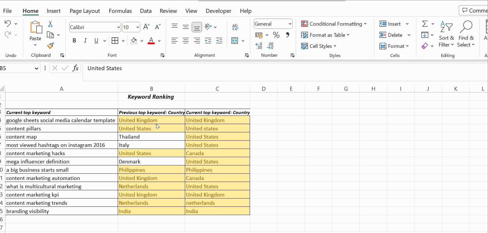 Ensuring Data Consistency with Excel Column Comparison
2. Methods for Comparing Columns in Excel
Excel offers several methods for comparing columns, each with its strengths and weaknesses. The best method for you will depend on the size of your dataset, the type of comparison you need to perform, and your comfort level with Excel formulas and features.
2.1. Using the Equals Operator (=)
The simplest way to compare two columns is to use the equals operator (=). This method performs a row-by-row comparison and returns TRUE if the values in the two cells are identical, and FALSE otherwise.
2.1.1. How to Use the Equals Operator
- Set up your data: Ensure the two columns you want to compare are adjacent to each other in your spreadsheet.
- Create a comparison column: In the first empty column next to your data, enter the formula
=A1=B1in the first cell (assuming your data starts in columns A and B). - Apply the formula to the entire column: Drag the fill handle (the small square at the bottom-right of the cell) down to apply the formula to all the rows you want to compare.
- Interpret the results: Excel will display TRUE for rows where the values in columns A and B match, and FALSE where they don’t.
2.1.2. Example
| Column A (IDs) | Column B (IDs) | Column C (Comparison) |
|---|---|---|
| 123 | 123 | TRUE |
| 456 | 789 | FALSE |
| 789 | 789 | TRUE |
| 101 | 111 | FALSE |
2.1.3. Advantages
- Simple and easy to use: Requires no advanced Excel knowledge.
- Fast for small datasets: Works well when you only need to compare a few rows.
2.1.4. Disadvantages
- Case-sensitive: Treats “Apple” and “apple” as different values.
- Doesn’t provide detailed information: Only tells you if the values match or not, not what the differences are.
- Not suitable for large datasets: Can be slow and cumbersome when dealing with thousands of rows.
2.2. Using the IF Function
The IF function allows you to perform a logical test and return one value if the test is TRUE and another value if the test is FALSE. This can be used to create more descriptive comparisons than the equals operator.
2.2.1. How to Use the IF Function
- Set up your data: As with the equals operator, ensure your columns are adjacent.
- Create a comparison column: In the first empty column, enter the formula
=IF(A1=B1, "Match", "No Match")in the first cell. - Apply the formula: Drag the fill handle down to apply the formula to all rows.
- Interpret the results: Excel will display “Match” for rows where the values are identical, and “No Match” where they differ.
2.2.2. Example
| Column A (Names) | Column B (Names) | Column C (Comparison) |
|---|---|---|
| John | John | Match |
| Jane | Janet | No Match |
| Peter | Peter | Match |
| Alice | Alicia | No Match |
2.2.3. Advantages
- More descriptive results: Allows you to display custom messages like “Match” and “No Match”.
- Easy to understand: The IF function is relatively straightforward to grasp.
2.2.4. Disadvantages
- Case-sensitive: Like the equals operator, it distinguishes between uppercase and lowercase letters.
- Still doesn’t provide detailed information: Only indicates whether the values match, not the nature of the differences.
- Not ideal for large datasets: Can be slow for very large spreadsheets.
2.3. Using the EXACT Function
The EXACT function is specifically designed to compare two text strings and returns TRUE only if they are exactly the same, including case.
2.3.1. How to Use the EXACT Function
- Set up your data: Make sure the columns you want to compare are next to each other.
- Create a comparison column: In the first cell of the new column, enter the formula
=IF(EXACT(A1, B1), "Match", "No Match"). - Apply the formula: Drag the fill handle down to apply the formula to all rows.
- Interpret the results: Excel will display “Match” only if the text strings are identical, including case.
2.3.2. Example
| Column A (Emails) | Column B (Emails) | Column C (Comparison) |
|---|---|---|
| [email protected] | [email protected] | Match |
| [email protected] | [email protected] | No Match |
| [email protected] | [email protected] | Match |
| [email protected] | [email protected] | No Match |
2.3.3. Advantages
- Case-sensitive: Ensures that the comparison takes case into account.
- Precise: Only returns “Match” if the strings are exactly the same.
2.3.4. Disadvantages
- Limited to text strings: Cannot be used to compare numbers or other data types directly.
- Still doesn’t provide detailed information: Only indicates whether the strings are exactly the same.
2.4. Using Conditional Formatting
Conditional formatting allows you to highlight cells based on certain criteria. This can be used to visually identify matching or mismatching values in two columns.
2.4.1. How to Use Conditional Formatting
- Select the columns: Select the two columns you want to compare.
- Open Conditional Formatting: Go to the Home tab, click on Conditional Formatting, then Highlight Cells Rules, and choose Duplicate Values.
- Choose formatting: In the dialog box, choose whether you want to highlight duplicate or unique values, and select a formatting style (e.g., fill color, text color).
- Apply the formatting: Click OK to apply the conditional formatting.
2.4.2. Example
| Column A (Products) | Column B (Products) |
|---|---|
| Apple | Apple |
| Banana | Orange |
| Orange | Grape |
| Grape | Banana |
In this example, if you choose to highlight duplicate values, “Apple” would be highlighted in both columns because it appears in both. If you choose to highlight unique values, “Banana,” “Orange,” and “Grape” would be highlighted in both columns because they each appear only once in the selected range.
2.4.3. Advantages
- Visual: Provides a quick visual representation of matching or mismatching values.
- Easy to set up: Requires no formulas.
2.4.4. Disadvantages
- No detailed information: Doesn’t tell you what the differences are, just that they exist.
- Can be overwhelming: If you have a lot of differences, the highlighting can become difficult to interpret.
- Doesn’t create a separate comparison column: Highlights the original data, which may not be desirable in all cases.
2.5. Using the VLOOKUP Function
The VLOOKUP function searches for a value in the first column of a range and returns a value from a specified column in the same row. This can be used to compare two columns and identify values that exist in one column but not in the other.
2.5.1. How to Use the VLOOKUP Function
- Set up your data: Ensure you have two columns to compare.
- Create a comparison column: In the first cell of the new column, enter the formula
=IF(ISNA(VLOOKUP(A1,B:B,1,FALSE)),"Not Found","Found"). - Apply the formula: Drag the fill handle down to apply the formula to all rows in column A.
- Interpret the results: The formula searches for the value in A1 within column B. If the value is found, the formula returns “Found”; otherwise, it returns “Not Found.”
2.5.2. Example
| Column A (List 1) | Column B (List 2) | Column C (Comparison) |
|---|---|---|
| Item1 | Item3 | Not Found |
| Item2 | Item2 | Found |
| Item3 | Item5 | Not Found |
| Item4 | Item4 | Found |
| Item5 | Item1 | Not Found |
In this example, VLOOKUP is used to check if each item in Column A exists in Column B. The results in Column C indicate whether each item from Column A was found in Column B.
2.5.3. Advantages
- Identifies missing values: Can quickly find values that exist in one column but not in the other.
- Flexible: Can be used to compare columns in different worksheets or even different workbooks.
2.5.4. Disadvantages
- Can be slow: VLOOKUP can be slow for large datasets.
- Requires understanding of VLOOKUP: Can be confusing for users who are not familiar with the function.
- Only finds the first match: If a value appears multiple times in the lookup column, VLOOKUP will only find the first instance.
2.6. Using the MATCH Function
The MATCH function searches for a specified item in a range of cells and returns the relative position of that item in the range. You can use it to see if a value from one column exists in another column and get its position.
2.6.1. How to Use the MATCH Function
- Set up your data: Ensure you have two columns to compare.
- Create a comparison column: In the first cell of the new column, enter the formula
=IF(ISNA(MATCH(A1,B:B,0)),"Not Found","Found"). - Apply the formula: Drag the fill handle down to apply the formula to all rows in column A.
- Interpret the results: The formula searches for the value in A1 within column B. If the value is found, the formula returns “Found”; otherwise, it returns “Not Found.”
2.6.2. Example
| Column A (List 1) | Column B (List 2) | Column C (Comparison) |
|---|---|---|
| Item1 | Item3 | Not Found |
| Item2 | Item2 | Found |
| Item3 | Item5 | Not Found |
| Item4 | Item4 | Found |
| Item5 | Item1 | Not Found |
In this example, MATCH is used to check if each item in Column A exists in Column B. The results in Column C indicate whether each item from Column A was found in Column B.
2.6.3. Advantages
- More flexible than VLOOKUP: Doesn’t require the lookup value to be in the first column of the range.
- Returns the position of the match: Can be useful for further analysis.
2.6.4. Disadvantages
- Can be slow: MATCH can be slow for large datasets.
- Requires understanding of MATCH: Can be confusing for users who are not familiar with the function.
- Only finds the first match: If a value appears multiple times in the lookup column, MATCH will only find the first instance.
2.7. Combining Functions for Complex Comparisons
Excel’s power lies in its ability to combine functions to perform complex comparisons. For example, you can combine the IF, AND, and EXACT functions to perform a case-sensitive comparison of multiple columns.
2.7.1. Example: Case-Sensitive Comparison of Multiple Columns
Suppose you have three columns of data (A, B, and C) and you want to identify rows where all three columns have the exact same value (including case). You could use the following formula:
=IF(AND(EXACT(A1, B1), EXACT(A1, C1)), "Match", "No Match")
This formula first uses the EXACT function to compare the values in columns A and B, and then again to compare the values in columns A and C. The AND function ensures that both comparisons return TRUE before the IF function returns “Match”.
2.7.2. Advantages
- Highly flexible: Allows you to create custom comparisons tailored to your specific needs.
- Powerful: Can perform complex comparisons that would be difficult or impossible to do with simple functions.
2.7.3. Disadvantages
- Requires advanced Excel knowledge: Can be challenging for users who are not familiar with Excel’s functions and syntax.
- Can be difficult to debug: Complex formulas can be hard to troubleshoot if they don’t work as expected.
3. Step-by-Step Examples
Let’s walk through some step-by-step examples of how to compare columns in Excel using the methods described above.
3.1. Example 1: Identifying Duplicate Email Addresses
Suppose you have a list of email addresses in column A and you want to identify any duplicate addresses.
- Select column A.
- Go to Home > Conditional Formatting > Highlight Cells Rules > Duplicate Values.
- Choose a formatting style (e.g., fill with red).
- Click OK.
Excel will highlight all duplicate email addresses in column A, making them easy to spot.
3.2. Example 2: Comparing Product Lists from Two Suppliers
Suppose you have a list of products from Supplier A in column A and a list of products from Supplier B in column B. You want to identify products that are offered by both suppliers.
- In column C, enter the formula
=IF(ISNA(VLOOKUP(A1,B:B,1,FALSE)),"Not Found","Found"). - Drag the fill handle down to apply the formula to all rows in column A.
- Filter column C to show only “Found” values.
Excel will show you the products that are offered by both Supplier A and Supplier B.
3.3. Example 3: Performing a Case-Sensitive Comparison of Names
Suppose you have a list of names in column A and a list of names in column B. You want to identify rows where the names are exactly the same, including case.
- In column C, enter the formula
=IF(EXACT(A1, B1), "Match", "No Match"). - Drag the fill handle down to apply the formula to all rows.
Excel will show you the rows where the names in columns A and B are exactly the same.
4. Optimizing Performance for Large Datasets
Comparing columns in Excel can be slow for large datasets. Here are some tips to optimize performance:
4.1. Use Formulas Efficiently
- Avoid volatile functions: Volatile functions (e.g., NOW(), RAND()) recalculate every time the spreadsheet changes, which can slow things down.
- Use array formulas sparingly: Array formulas can be powerful, but they can also be slow.
- Use helper columns: Sometimes, breaking a complex formula into smaller parts using helper columns can improve performance.
4.2. Disable Automatic Calculation
Turning off automatic calculation can prevent Excel from recalculating the entire spreadsheet every time you make a change. To do this:
- Go to Formulas > Calculation Options.
- Select Manual.
Remember to press F9 to manually recalculate the spreadsheet when you’re done making changes.
4.3. Use Excel Tables
Excel tables can improve performance by automatically managing formulas and data ranges. To create an Excel table:
- Select your data.
- Go to Insert > Table.
- Check the “My table has headers” box if your data has headers.
- Click OK.
4.4. Consider Using Power Query
Power Query is a powerful data transformation and analysis tool that is built into Excel. It can be used to perform complex comparisons and transformations on large datasets.
5. The Importance of Choosing the Right Comparison Method
Selecting the appropriate method for comparing columns in Excel is critical for accuracy and efficiency. Each technique, from the basic equals operator to more complex functions like VLOOKUP and conditional formatting, has its own strengths and limitations.
5.1. Matching the Method to Your Data
The nature of your data should guide your choice of comparison method. For instance, if you’re dealing with text strings where case sensitivity matters, the EXACT function is invaluable. On the other hand, if you need a quick visual overview of duplicate entries, conditional formatting might be the best option.
5.2. Balancing Speed and Accuracy
For large datasets, the speed of the comparison method becomes a significant factor. While functions like VLOOKUP are powerful, they can be slower than simpler methods like the equals operator. It’s essential to strike a balance between speed and the level of detail required for your comparison.
5.3. Understanding the Limitations
Each method has limitations that you should be aware of. The equals operator, for example, doesn’t provide detailed information about mismatches. VLOOKUP only finds the first match, which might not be sufficient in all scenarios. Being aware of these limitations will help you choose the most appropriate method and interpret the results accurately.
5.4. Adaptability and Flexibility
Your needs might change over time, so it’s essential to choose a method that is adaptable and flexible. Combining functions, for instance, allows you to create custom comparisons tailored to your specific requirements. This adaptability ensures that you can always find the right method for your data, no matter how complex it might be.
5.5. The Role of Excel Expertise
Your level of Excel expertise will also influence your choice of method. While complex functions like VLOOKUP can be powerful, they require a deeper understanding of Excel’s capabilities. If you’re new to Excel, starting with simpler methods like the equals operator or conditional formatting might be more manageable.
6. Advanced Tips and Tricks for Column Comparison
Once you’re comfortable with the basic methods for comparing columns in Excel, you can start exploring some advanced tips and tricks to enhance your skills.
6.1. Using Array Formulas for Complex Comparisons
Array formulas allow you to perform calculations on multiple values at once. They can be used to perform complex comparisons that would be difficult or impossible to do with regular formulas.
For example, suppose you want to count the number of rows where the values in columns A and B are different. You could use the following array formula:
=SUM(IF(A1:A100<>B1:B100,1,0))
To enter an array formula, you must press Ctrl+Shift+Enter instead of just Enter.
6.2. Using the INDEX Function with MATCH
The INDEX function returns a value from a specified row and column in a range. It can be used with the MATCH function to perform more flexible lookups.
For example, suppose you have a table of data with customer IDs in column A and customer names in column B. You want to find the customer name for a specific customer ID. You could use the following formula:
=INDEX(B:B,MATCH(customer_id,A:A,0))
Where customer_id is the customer ID you want to look up.
6.3. Using the CHOOSE Function for Multiple Conditions
The CHOOSE function returns a value from a list of values based on a specified index number. It can be used to create formulas with multiple conditions.
For example, suppose you want to compare the values in columns A and B and return “Match” if they are the same, “Different” if they are different, and “Empty” if either cell is empty. You could use the following formula:
=CHOOSE(IF(ISBLANK(A1)+ISBLANK(B1),3,IF(A1=B1,1,2)),"Match","Different","Empty")
6.4. Creating Custom Functions with VBA
If you need to perform a specific type of comparison that is not easily done with Excel’s built-in functions, you can create a custom function using VBA (Visual Basic for Applications).
To create a custom function:
- Press Alt+F11 to open the VBA editor.
- Go to Insert > Module.
- Enter your VBA code.
- Close the VBA editor.
You can then use your custom function in your spreadsheet just like any other Excel function.
6.5. Using Power BI for Advanced Data Analysis
For very large datasets or complex comparisons, you may want to consider using Power BI, Microsoft’s business intelligence tool. Power BI allows you to connect to various data sources, transform and analyze data, and create interactive reports and dashboards.
7. Real-World Applications of Column Comparison
The ability to compare columns in Excel has numerous real-world applications across various industries and fields.
7.1. Finance
In finance, column comparison is used for:
- Reconciling bank statements: Comparing transactions in a bank statement with transactions in a company’s accounting system.
- Auditing financial data: Comparing data from different sources to identify discrepancies and errors.
- Analyzing investment performance: Comparing the performance of different investments over time.
7.2. Marketing
In marketing, column comparison is used for:
- Segmenting customer data: Comparing customer data from different sources to identify customer segments.
- Measuring campaign effectiveness: Comparing the results of different marketing campaigns to determine which ones are most effective.
- Personalizing marketing messages: Comparing customer data to create personalized marketing messages.
7.3. Operations
In operations, column comparison is used for:
- Managing inventory: Comparing inventory levels with sales data to identify slow-moving or obsolete items.
- Optimizing supply chain: Comparing data from different suppliers to identify the most cost-effective and reliable suppliers.
- Improving process efficiency: Comparing data from different stages of a process to identify bottlenecks and inefficiencies.
7.4. Human Resources
In human resources, column comparison is used for:
- Tracking employee performance: Comparing employee performance data over time to identify trends and areas for improvement.
- Managing compensation: Comparing employee salaries with industry benchmarks to ensure fair compensation.
- Recruiting new employees: Comparing candidate data to identify the best candidates for a job.
7.5. Healthcare
In healthcare, column comparison is used for:
- Analyzing patient data: Comparing patient data from different sources to identify patterns and trends.
- Managing clinical trials: Comparing data from different treatment groups to determine the effectiveness of a new treatment.
- Improving patient safety: Comparing data from different hospitals to identify best practices for patient safety.
8. Common Mistakes to Avoid When Comparing Columns
Even with the right methods and techniques, it’s easy to make mistakes when comparing columns in Excel. Here are some common mistakes to avoid:
8.1. Not Checking for Data Type Consistency
Before comparing columns, make sure that the data types are consistent. For example, if one column contains numbers formatted as text, and the other column contains numbers formatted as numbers, the comparison may not work correctly.
To check the data type of a cell, select the cell and look at the Number format in the Home tab.
8.2. Ignoring Case Sensitivity
As mentioned earlier, some comparison methods are case-sensitive, while others are not. Make sure you are using the appropriate method for your data.
If you need to perform a case-insensitive comparison, you can use the UPPER or LOWER functions to convert the data to the same case before comparing.
8.3. Not Handling Errors Correctly
If your formulas return errors, the comparison may not work correctly. Make sure you are handling errors correctly using functions like IFERROR or ISERROR.
8.4. Not Testing Your Formulas
Before using your formulas on a large dataset, test them on a small sample to make sure they are working correctly.
8.5. Not Documenting Your Formulas
It’s always a good idea to document your formulas so that you can remember what they do later on. You can add comments to your formulas using the N function.
9. Frequently Asked Questions (FAQ)
1. How can I compare two columns in Excel to find the differences?
You can use the IF function combined with the <> (not equal to) operator. For example, =IF(A1<>B1, "Different", "Same") will return “Different” if the values in A1 and B1 are not the same, and “Same” if they are.
2. How do I compare two columns and highlight the matching cells?
Use conditional formatting. Select both columns, go to Home > Conditional Formatting > Highlight Cells Rules > Duplicate Values. Choose the formatting you want to apply to the matching cells.
3. Is there a way to compare two columns and return a value from a third column if there is a match?
Yes, use the VLOOKUP function. For example, if you want to compare column A with column B and return a value from column C when there’s a match, use the formula =IFERROR(VLOOKUP(A1, B:C, 2, FALSE), "No Match").
4. How can I compare two columns in different Excel sheets?
You can use the same formulas, but you need to reference the other sheet. For example, to compare A1 in Sheet1 with A1 in Sheet2, use =IF(Sheet1!A1=Sheet2!A1, "Match", "No Match").
5. Can I compare two columns ignoring case sensitivity?
Yes, use the UPPER or LOWER functions to convert both columns to the same case before comparing. For example, =IF(UPPER(A1)=UPPER(B1), "Match", "No Match").
6. How do I compare two columns and identify unique values in each column?
Use conditional formatting with a formula. For example, to highlight unique values in column A compared to column B, select column A, go to Conditional Formatting > New Rule > Use a formula to determine which cells to format and enter the formula =COUNTIF(B:B, A1)=0.
7. How can I compare multiple columns in Excel?
You can use the AND function within an IF statement. For example, to check if A1, B1, and C1 are all equal, use =IF(AND(A1=B1, B1=C1), "All Match", "Not All Match").
8. How do I compare two columns to find missing values?
Use the MATCH function to see if values from one column exist in the other. For example, to find values in column A that are not in column B, use =IF(ISNA(MATCH(A1, B:B, 0)), "Missing", "Found").
9. How can I optimize performance when comparing large columns in Excel?
Disable automatic calculations, use array formulas sparingly, and consider using Excel tables or Power Query.
10. What is the difference between using the EXACT function and the = operator to compare columns?
The EXACT function is case-sensitive and checks for an exact match, while the = operator is not case-sensitive. EXACT is more precise, while = is more general.
10. Conclusion: Mastering Column Comparison for Data Excellence
Comparing columns in Excel is a crucial skill for anyone working with data. By mastering the various methods and techniques described in this guide, you can improve your data accuracy, efficiency, and decision-making. Remember to choose the right method for your specific needs, avoid common mistakes, and optimize performance for large datasets.
At COMPARE.EDU.VN, we are dedicated to providing you with the knowledge and resources you need to excel in data analysis. Whether you are a beginner or an experienced Excel user, we hope this guide has helped you enhance your column comparison skills. Explore our website at COMPARE.EDU.VN for more articles, tutorials, and resources to help you master Excel and other data analysis tools.
Need help comparing complex datasets? Contact us at 333 Comparison Plaza, Choice City, CA 90210, United States or via Whatsapp at +1 (626) 555-9090. Let compare.edu.vn be your partner in data excellence.