How Do You Compare Columns In Excel For Data Analysis?

How Do You Compare Columns In Excel? Comparing columns in Excel is a fundamental task for data analysis, enabling you to identify matches, differences, and unique entries, and COMPARE.EDU.VN offers detailed guides to simplify this process. Using Excel column comparison techniques such as conditional formatting, formulas, and functions will help you effectively compare data sets, identify discrepancies, and ensure data integrity. Discover the best methods for comparing columns for duplicate values, and data validation to improve your spreadsheet skills.

1. Why Comparing Columns in Excel is Essential

Excel is a robust tool for data storage, manipulation, and analysis. While it may not be the best for complex calculations, its versatility in text formatting makes it an invaluable asset. Features like column comparison empower data analysts to make well-informed decisions based on data. Comparing columns within the same or different spreadsheets is essential for various reasons:

Data Validation: Verifying the accuracy and consistency of data across different sources.
Identifying Discrepancies: Pinpointing differences in datasets to detect errors or anomalies.
Duplicate Detection: Finding and removing duplicate entries to maintain data integrity.
Data Integration: Merging data from different sources while ensuring consistency.

Manual comparison is time-consuming and prone to errors. Excel provides several methods to streamline this process, displaying results as TRUE/FALSE, Match/Not Match, or custom messages, enhancing data analysis efficiency.

2. Methods to Compare Columns in Excel

Depending on your specific needs, Excel offers various methods to compare columns effectively:

Highlighting unique or duplicate values using functions.
Displaying unique or duplicate cells using conditional formatting or formulas.
Performing row-by-row comparisons.
Using LOOKUP formulas.

Let’s delve into each method with detailed explanations and examples.

3. Comparing Two Columns Using the Equals Operator

The equals operator (=) provides a simple way to compare two columns on a row-by-row basis, returning “TRUE” if the values match and “FALSE” if they differ.

3.1. Step-by-Step Guide

Open your Excel spreadsheet: Ensure the columns you want to compare are adjacent to each other.
Create a new column for the results: This column will display whether the rows match or not.
Enter the formula: In the first cell of the results column (e.g., D4), enter the formula =B4=C4. This formula compares the values in cells B4 and C4.
Press Enter: The cell will display either “TRUE” or “FALSE” based on whether the values match.
Drag the formula down: Click and drag the bottom-right corner of the cell down to apply the formula to the rest of the rows in the column.

3.2. Example

Consider two columns, B and C, containing country names. To compare if the country names in each row match, use the following steps:

Row	Column B (Country 1)	Column C (Country 2)	Column D (Result)	Formula
4	USA	USA	TRUE	=B4=C4
5	Canada	Canada	TRUE	=B5=C5
6	UK	Germany	FALSE	=B6=C6
7	France	France	TRUE	=B7=C7
8	Japan	Japan	TRUE	=B8=C8

In this example, column D displays “TRUE” for rows where the country names in columns B and C match, and “FALSE” where they differ.

4. Comparing Two Columns Using the IF Condition

The IF condition allows you to return custom messages like “Match” or “Not Match” instead of the default “TRUE” or “FALSE.”

4.1. Basic IF Condition

The formula =IF(B4=C4,"Yes"," ") returns “Yes” for matching values and leaves the cell blank for non-matching values.

4.2. Step-by-Step Guide

Open your Excel spreadsheet: Ensure the columns you want to compare are adjacent to each other.
Create a new column for the results: This column will display custom messages based on the comparison.
Enter the formula: In the first cell of the results column (e.g., D4), enter the formula =IF(B4=C4,"Yes"," ").
Press Enter: The cell will display “Yes” if the values in cells B4 and C4 match, and remain blank if they don’t.
Drag the formula down: Click and drag the bottom-right corner of the cell down to apply the formula to the rest of the rows in the column.

4.3. Enhanced IF Condition for Mismatches

To display a specific message for mismatches, use the formula =IF(B4=C4,"Yes","No"), which returns “Yes” for matching values and “No” for non-matching values.

4.4. Step-by-Step Guide

Open your Excel spreadsheet: Ensure the columns you want to compare are adjacent to each other.
Create a new column for the results: This column will display custom messages based on the comparison.
Enter the formula: In the first cell of the results column (e.g., D4), enter the formula =IF(B4=C4,"Yes","No").
Press Enter: The cell will display “Yes” if the values in cells B4 and C4 match, and “No” if they don’t.
Drag the formula down: Click and drag the bottom-right corner of the cell down to apply the formula to the rest of the rows in the column.

4.5. Identifying Differences

To identify differences between two columns, replace the equals sign (=) with the non-equality sign (<>). The formula =IF(B4<>C4,"Match","Not a Match") returns “Match” if the values are different and “Not a Match” if they are the same.

4.6. Step-by-Step Guide

Open your Excel spreadsheet: Ensure the columns you want to compare are adjacent to each other.
Create a new column for the results: This column will display custom messages based on the comparison.
Enter the formula: In the first cell of the results column (e.g., D4), enter the formula =IF(B4<>C4,"Match","Not a Match").
Press Enter: The cell will display “Match” if the values in cells B4 and C4 are different, and “Not a Match” if they are the same.
Drag the formula down: Click and drag the bottom-right corner of the cell down to apply the formula to the rest of the rows in the column.

4.7. Example

Row	Column B (Data 1)	Column C (Data 2)	Column D (Result)	Formula
4	Apple	Apple	Not a Match	=IF(B4<>C4,”Match”,”Not a Match”)
5	Banana	Orange	Match	=IF(B5<>C5,”Match”,”Not a Match”)
6	Cherry	Cherry	Not a Match	=IF(B6<>C6,”Match”,”Not a Match”)
7	Date	Fig	Match	=IF(B7<>C7,”Match”,”Not a Match”)
8	Grape	Grape	Not a Match	=IF(B8<>C8,”Match”,”Not a Match”)

In this example, column D displays “Match” for rows where the data in columns B and C are different, and “Not a Match” where they are the same.

5. Comparing Two Columns Using the EXACT() Function

The EXACT() function ensures case-sensitive comparisons, which means it distinguishes between uppercase and lowercase letters. This is particularly useful when capitalization matters in your data.

5.1. Syntax and Usage

The syntax for the EXACT() function is =EXACT(text1, text2), where text1 and text2 are the two strings you want to compare. The function returns “TRUE” if the strings are exactly the same, including case, and “FALSE” otherwise.

5.2. Integrating EXACT() with IF()

To use EXACT() in conjunction with IF(), use the formula =IF(EXACT(B4,C4), "Match", "Mismatched"). This formula returns “Match” only if the values in cells B4 and C4 are identical, including capitalization.

5.3. Step-by-Step Guide

Open your Excel spreadsheet: Ensure the columns you want to compare are adjacent to each other.
Create a new column for the results: This column will display custom messages based on the comparison.
Enter the formula: In the first cell of the results column (e.g., D4), enter the formula =IF(EXACT(B4,C4), "Match", "Mismatched").
Press Enter: The cell will display “Match” if the values in cells B4 and C4 are exactly the same, and “Mismatched” if they are not.
Drag the formula down: Click and drag the bottom-right corner of the cell down to apply the formula to the rest of the rows in the column.

5.4. Example

Row	Column B (Country 1)	Column C (Country 2)	Column D (Result)	Formula
4	USA	USA	Match	=IF(EXACT(B4,C4), “Match”, “Mismatched”)
5	Netherlands	netherlands	Mismatched	=IF(EXACT(B5,C5), “Match”, “Mismatched”)
6	UK	Germany	Mismatched	=IF(EXACT(B6,C6), “Match”, “Mismatched”)
7	France	France	Match	=IF(EXACT(B7,C7), “Match”, “Mismatched”)
8	Japan	Japan	Match	=IF(EXACT(B8,C8), “Match”, “Mismatched”)

In this example, column D displays “Mismatched” for rows where the capitalization in columns B and C differs, even if the country names are the same.

5.5. Execution of the Formula

The EXACT() function is executed first, and its result (TRUE or FALSE) is then passed to the IF() function. If EXACT() returns TRUE, the IF() function returns “Match”; otherwise, it returns “Mismatched.”

6. Comparing Two Columns Using Conditional Formatting

Conditional formatting allows you to highlight unique or duplicate values directly within the columns, without needing a third column for results.

6.1. Highlighting Duplicate Values

Select the columns: Click and drag to select the columns you want to compare.
Open Conditional Formatting: Go to Home → Styles → Conditional Formatting → Highlight Cell Rules → Duplicate Values.
Choose Formatting: In the dialog box, choose “Duplicate” from the drop-down menu.
Select a Format: Choose a formatting option, such as filling the cells with a color, changing the text color, or changing the cell border.
Click OK: Excel will highlight all duplicate values in the selected columns.

6.2. Highlighting Unique Values

Select the columns: Click and drag to select the columns you want to compare.
Open Conditional Formatting: Go to Home → Styles → Conditional Formatting → Highlight Cell Rules → Duplicate Values.
Choose Formatting: In the dialog box, choose “Unique” from the drop-down menu.
Select a Format: Choose a formatting option, such as filling the cells with a color, changing the text color, or changing the cell border.
Click OK: Excel will highlight all unique values in the selected columns.

6.3. Custom Formatting

For more specific formatting, choose “Custom Format” in the dialog box. This option allows you to select a custom color or style for the highlighted cells.

6.4. Clearing Conditional Formatting

To remove conditional formatting, click Conditional Formatting → Clear Rules → Clear Rules from Selected Cells.

6.5. Example

Suppose you have two columns, B and C, with the following data:

Row	Column B	Column C
4	Apple	Banana
5	Banana	Orange
6	Cherry	Cherry
7	Date	Fig
8	Grape	Grape

To highlight duplicate values (values present in both columns):

Select columns B and C.
Go to Home → Conditional Formatting → Highlight Cell Rules → Duplicate Values.
Choose “Duplicate” and select a color (e.g., green fill).
Click OK.

The result will highlight “Cherry” and “Grape” in both columns, indicating they are present in both datasets.

7. Using Lookup Functions to Compare Two Columns

Lookup functions like VLOOKUP, HLOOKUP, and XLOOKUP search for a value in a row or column and return a corresponding value from another row or column. These functions are useful for comparing columns and identifying matches or differences.

7.1. VLOOKUP Function

The VLOOKUP (Vertical Lookup) function searches for a value in the first column of a range and returns a value in the same row from another column.

7.2. Syntax

The syntax for VLOOKUP is =VLOOKUP(lookup_value, table_array, col_index_num, [range_lookup]).

lookup_value: The value you want to search for.
table_array: The range of cells where you want to search.
col_index_num: The column number in the table_array from which to return a value.
range_lookup: A logical value (TRUE or FALSE) that specifies whether to find an approximate or exact match. Use FALSE for exact matches.

7.3. Example

Suppose you have two columns: A (Product IDs) and B (Product Names). You want to compare these columns to another column, D (New Product IDs), and return the corresponding Product Names from column B if there is a match.

Row	Column A (Product IDs)	Column B (Product Names)	Column D (New Product IDs)	Column E (Result)
4	101	Apple	102	#N/A
5	102	Banana	105	#N/A
6	103	Cherry	103	Cherry
7	104	Date	101	Apple
8	105	Grape

To compare column D with column A and return the corresponding Product Names from column B, enter the following formula in cell E4:

=VLOOKUP(D4, A4:B8, 2, FALSE)

Drag the formula down to apply it to the rest of the rows in column E.

The formula works as follows:

VLOOKUP(D4, A4:B8, 2, FALSE): Searches for the value in cell D4 within the range A4:B8. If a match is found, it returns the value from the second column (Product Names) in the same row.

The results in column E will show the corresponding Product Names for matching Product IDs, and #N/A for non-matching Product IDs.

7.4. Absolute References

To prevent the table_array from changing when you drag the formula down, use absolute references (e.g., $A$4:$B$8). The formula becomes:

=VLOOKUP(D4, $A$4:$B$8, 2, FALSE)

7.5. Handling Errors

To handle #N/A errors, use the IFERROR function. The formula becomes:

=IFERROR(VLOOKUP(D4, $A$4:$B$8, 2, FALSE), "Not Found")

This formula will display “Not Found” instead of #N/A for non-matching Product IDs.

8. Comparing Multiple Columns

Comparing three or more columns involves using a combination of IF() and AND() or OR() statements.

8.1. Finding Matches in All Columns

To find rows where all columns match, use the AND() function within an IF() statement. The formula is =IF(AND(A2=B2, A2=C2), "Full Match", "").

8.2. Step-by-Step Guide

Open your Excel spreadsheet: Ensure the columns you want to compare are adjacent to each other.
Create a new column for the results: This column will display whether all columns match in each row.
Enter the formula: In the first cell of the results column (e.g., D2), enter the formula =IF(AND(A2=B2, A2=C2), "Full Match", "").
Press Enter: The cell will display “Full Match” if the values in cells A2, B2, and C2 are the same, and remain blank if they are not.
Drag the formula down: Click and drag the bottom-right corner of the cell down to apply the formula to the rest of the rows in the column.

8.3. Finding Matches in Any Two Columns

To find rows where any two columns match, use the OR() function within an IF() statement. The formula is =IF(OR(A2=B2, B2=C2, A2=C2), "Match", "").

8.4. Step-by-Step Guide

Open your Excel spreadsheet: Ensure the columns you want to compare are adjacent to each other.
Create a new column for the results: This column will display whether any two columns match in each row.
Enter the formula: In the first cell of the results column (e.g., D2), enter the formula =IF(OR(A2=B2, B2=C2, A2=C2), "Match", "").
Press Enter: The cell will display “Match” if any two of the values in cells A2, B2, and C2 are the same, and remain blank if none match.
Drag the formula down: Click and drag the bottom-right corner of the cell down to apply the formula to the rest of the rows in the column.

8.5. Example

Consider three columns, A, B, and C, with the following data:

Row	Column A	Column B	Column C	Column D (Full Match)	Column E (Any Match)
2	Apple	Apple	Apple	Full Match	Match
3	Banana	Orange	Cherry
4	Cherry	Cherry	Date		Match
5	Date	Fig	Date		Match
6	Grape	Grape	Grape	Full Match	Match

In this example:

Column D displays “Full Match” only when all three columns have the same value.
Column E displays “Match” when any two columns have the same value.

9. Advanced Techniques

9.1. Using Array Formulas

Array formulas can perform complex comparisons across multiple columns. For example, to count the number of matching values across multiple columns for each row, you can use an array formula.

Select a range of cells: Choose the range where you want the results to appear.
Enter the formula: Type the formula =(A1:A5=B1:B5)*(A1:A5=C1:C5) and press Ctrl+Shift+Enter. This creates an array formula.

This formula compares corresponding cells across columns A, B, and C, and returns an array of 1s and 0s, where 1 indicates a match and 0 indicates a mismatch.

9.2. Using Power Query

Power Query, also known as Get & Transform Data, is a powerful tool for data transformation and comparison. It allows you to import data from various sources, clean and transform it, and then compare columns using advanced techniques like merging and joining.

9.3. Using VBA (Visual Basic for Applications)

For highly customized comparisons, you can use VBA to write custom functions and macros. This allows you to define specific comparison criteria and automate complex tasks.

10. Optimizing Performance for Large Datasets

When working with large datasets in Excel, performance can become a concern. Here are some tips to optimize performance when comparing columns:

Use Efficient Formulas: Use simple formulas like = and IF() whenever possible, as they are faster than more complex functions like VLOOKUP().
Avoid Volatile Functions: Volatile functions like NOW() and TODAY() recalculate every time the worksheet changes, which can slow down performance. Avoid using them in your comparison formulas.
Use Helper Columns: Instead of using complex formulas that perform multiple operations in a single cell, break down the calculation into multiple helper columns. This can improve performance by reducing the complexity of each individual formula.
Disable Automatic Calculation: When making changes to a large dataset, disable automatic calculation by setting calculation mode to manual. This prevents Excel from recalculating the worksheet every time you make a change.
Use Excel Tables: Convert your data ranges into Excel Tables. Tables are designed to work efficiently with large datasets and can improve performance when filtering, sorting, and calculating data.
Use Indexing: If you need to perform lookups on a large dataset, consider using indexing techniques to speed up the lookup process. Indexing involves creating a separate table that maps lookup values to their corresponding row numbers.
Consider Using Alternatives: If you are working with extremely large datasets that exceed Excel’s capabilities, consider using alternative tools like databases (e.g., MySQL, PostgreSQL) or data processing frameworks (e.g., Apache Spark).

11. Common Mistakes to Avoid

Ignoring Case Sensitivity: Failing to account for case sensitivity when comparing text values can lead to incorrect results. Use the EXACT() function for case-sensitive comparisons.
Not Using Absolute References: Forgetting to use absolute references when dragging formulas can cause the comparison range to shift, resulting in incorrect results.
Misunderstanding Lookup Functions: Using the wrong parameters or syntax for lookup functions can lead to errors. Double-check the documentation and examples before using these functions.
Not Handling Errors: Failing to handle errors like #N/A can make your results difficult to interpret. Use the IFERROR function to display a custom message instead of errors.
Overcomplicating Formulas: Using overly complex formulas can make your worksheet difficult to understand and maintain. Break down complex calculations into multiple steps using helper columns.

12. FAQ

12.1. How do I compare two columns in Excel for differences?

Use the formula =IF(B4<>C4,"Match","Not a Match") to identify differences between two columns. This formula returns “Match” if the values are different and “Not a Match” if they are the same.

12.2. How do I compare two columns in Excel and highlight the differences?

Use conditional formatting to highlight the differences. Select the columns, then go to Home → Conditional Formatting → Highlight Cell Rules → Duplicate Values. Choose “Unique” to highlight the different values.

12.3. How do I compare two columns in Excel for matching values?

Use the formula =IF(B4=C4,"Yes","No") to identify matching values. This formula returns “Yes” if the values match and “No” if they don’t.

12.4. How can I compare two columns in Excel case-sensitively?

Use the EXACT() function in conjunction with the IF() function. The formula =IF(EXACT(B4,C4), "Match", "Mismatched") returns “Match” only if the values are identical, including capitalization.

12.5. How do I compare three or more columns in Excel?

Use a combination of IF() and AND() or OR() statements. For example, =IF(AND(A2=B2, A2=C2), "Full Match", "") finds matches in all columns, while =IF(OR(A2=B2, B2=C2, A2=C2), "Match", "") finds matches in any two columns.

12.6. What if I have a lot of columns to compare in Excel?

For a large number of columns, using VBA or Power Query might be more efficient. These tools can automate the process of comparing multiple columns and provide more advanced options for handling complex comparisons.

12.7. How can I visualize the differences between two columns in Excel?

Besides conditional formatting, you can create charts or graphs to visualize the differences. For example, you can create a bar chart comparing the values in each column or a scatter plot to identify outliers and discrepancies.

12.8. Can I compare columns in Excel on different sheets?

Yes, you can compare columns on different sheets by referencing the sheet names in your formulas. For example, to compare column A in Sheet1 with column A in Sheet2, you can use the formula =IF(Sheet1!A1=Sheet2!A1, "Match", "Not Match").

12.9. Is there a way to ignore blank cells when comparing columns in Excel?

Yes, you can modify your formulas to ignore blank cells by adding a condition to check if the cells are blank before comparing them. For example, you can use the formula =IF(AND(A1<>"", B1<>""), IF(A1=B1, "Match", "Not Match"), "") to ignore blank cells.

12.10. How do I compare dates in two columns in Excel?

You can compare dates in two columns using the same comparison operators as with other values. However, make sure that the dates are formatted correctly as dates in Excel. If the dates are stored as text, you may need to convert them to dates using the DATEVALUE function before comparing them.

13. Conclusion

Comparing columns in Excel is a critical skill for data analysis, enabling you to validate data, identify discrepancies, and maintain data integrity. Whether you’re using the equals operator, IF conditions, the EXACT() function, conditional formatting, or lookup functions, Excel provides a range of tools to suit your needs. By understanding and applying these methods, you can efficiently compare columns and make informed decisions based on your data.

For more detailed guides and advanced techniques on data analysis in Excel, visit COMPARE.EDU.VN. Our comprehensive resources will help you master Excel and unlock the full potential of your data.

Need more help with comparing data or making the right choices? Contact us at 333 Comparison Plaza, Choice City, CA 90210, United States, or reach out via WhatsApp at +1 (626) 555-9090. Visit our website at compare.edu.vn for expert comparisons and detailed guides.

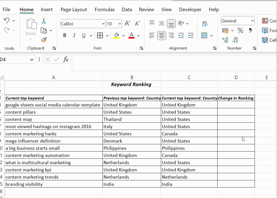Compare Two Columns in Excel using IF Condition