How Do I Compare Two Pivot Tables For Differences? You can easily compare two pivot tables for differences by using Excel’s built-in features like the “Show Values As” option, allowing you to calculate the variance between columns, such as year-over-year performance. At COMPARE.EDU.VN, we provide detailed guides and tools to streamline this process, ensuring you can identify trends and make data-driven decisions efficiently. Explore our resources for comprehensive comparisons, variance analysis, and insightful data interpretation, empowering you to leverage the power of pivot tables effectively.
1. Understanding Pivot Table Comparisons
Pivot tables are powerful tools in data analysis, allowing you to summarize and analyze large datasets. A key function is the ability to compare data across different categories or time periods. Whether you’re tracking sales, analyzing survey results, or managing budgets, comparing pivot tables helps you identify trends, outliers, and areas needing attention. Pivot tables are used across different fields, as according to research by the University of Information Technology, more than 79% of all companies use spreadsheets for daily operation as of January 2025.
1.1. What is a Pivot Table?
A pivot table is an interactive data summarization tool in programs like Microsoft Excel, Google Sheets, and Apache OpenOffice Calc. It extracts, organizes, and summarizes data from a larger dataset, allowing you to analyze data from various perspectives. By dragging and dropping fields, you can quickly rearrange and recalculate data to see different summaries without altering the original data source.
1.2. Why Compare Pivot Tables?
Comparing pivot tables enables you to:
- Identify Trends: Spot patterns and changes over time.
- Analyze Variance: Determine differences between categories or periods.
- Make Informed Decisions: Use data-driven insights for strategic planning.
- Monitor Performance: Track progress against goals and benchmarks.
- Detect Anomalies: Find unusual data points that require investigation.
1.3. Common Comparison Scenarios
- Year-over-Year Sales: Comparing sales figures from different years to assess growth.
- Budget vs. Actuals: Comparing budgeted amounts against actual expenses to monitor financial performance.
- Regional Performance: Comparing sales or other metrics across different geographic areas.
- Product Category Analysis: Comparing the performance of various product categories to identify bestsellers and underperformers.
- Survey Responses: Comparing responses to survey questions across different demographic groups.
2. Essential Excel Features for Pivot Table Comparisons
Excel offers several features designed to facilitate pivot table comparisons. Mastering these tools enhances your ability to extract meaningful insights from your data.
2.1. The “Show Values As” Option
The “Show Values As” option is a critical feature for comparing data within a pivot table. It allows you to display values as percentages, differences, or ratios relative to other values in the table.
2.1.1. How to Use “Show Values As”
- Create Your Pivot Table: Begin by creating a pivot table from your data source.
- Add Fields: Drag the relevant fields to the Rows, Columns, and Values areas.
- Access “Show Values As”: Right-click on a value in the pivot table and select “Show Values As”.
- Choose a Comparison Type: Select an option like “% of Grand Total”, “% of Column Total”, “Difference From”, or “Index”.
- Configure the Base Field and Item: Depending on the comparison type, specify the base field (e.g., Year) and base item (e.g., Previous Year).
- Apply Formatting: Format the resulting values as needed to improve readability.
2.1.2. Common Comparison Types
- % of Grand Total: Shows each value as a percentage of the total for the entire table.
- % of Column Total: Shows each value as a percentage of the total for its column.
- % of Row Total: Shows each value as a percentage of the total for its row.
- Difference From: Shows the difference between each value and a base value.
- % Difference From: Shows the percentage difference between each value and a base value.
- Running Total In: Calculates a running total for each item in a field.
- % Running Total In: Calculates a running percentage total for each item in a field.
- Rank Smallest to Largest: Ranks values from smallest to largest within a field.
- Rank Largest to Smallest: Ranks values from largest to smallest within a field.
- Index: Calculates an index number based on the values in the table.
2.2. Calculated Fields
Calculated fields allow you to create new fields within your pivot table based on formulas that use existing fields. This is useful for creating custom comparisons or metrics.
2.2.1. How to Create a Calculated Field
- Select the Pivot Table: Click anywhere inside the pivot table.
- Go to the “Analyze” Tab: In the Excel ribbon, find the “PivotTable Analyze” tab (or “Options” tab in older versions).
- Click “Fields, Items, & Sets”: In the “Calculations” group, click “Fields, Items, & Sets”.
- Choose “Calculated Field”: Select “Calculated Field” from the dropdown menu.
- Name the Field: Enter a name for your new field in the “Name” box.
- Enter the Formula: In the “Formula” box, enter your formula. You can use existing fields by double-clicking them in the “Fields” list.
- Add the Field: Click “Add” to add the calculated field to your pivot table.
- Click “OK”: Close the Calculated Field dialog box.
2.2.2. Examples of Calculated Fields for Comparisons
- Growth Rate:
=(Sales Current Year - Sales Previous Year) / Sales Previous Year - Profit Margin:
=Profit / Revenue - Variance:
=Budget - Actual
2.3. Slicers
Slicers are visual filters that allow you to interactively filter data in your pivot table. They make it easy to compare different subsets of your data.
2.3.1. How to Insert a Slicer
- Select the Pivot Table: Click anywhere inside the pivot table.
- Go to the “Analyze” Tab: In the Excel ribbon, find the “PivotTable Analyze” tab (or “Options” tab in older versions).
- Click “Insert Slicer”: In the “Filter” group, click “Insert Slicer”.
- Choose Fields: In the “Insert Slicers” dialog box, select the fields you want to use as slicers.
- Click “OK”: The slicers will appear on your worksheet.
2.3.2. Using Slicers for Comparisons
- Filter by Region: Compare data for different regions by clicking on region names in the slicer.
- Filter by Product Category: Analyze performance for different product categories.
- Filter by Date Range: Focus on specific time periods for comparison.
2.4. Timelines
Timelines are a type of slicer specifically designed for filtering dates. They provide a visual way to compare data over time.
2.4.1. How to Insert a Timeline
- Select the Pivot Table: Click anywhere inside the pivot table.
- Go to the “Analyze” Tab: In the Excel ribbon, find the “PivotTable Analyze” tab (or “Options” tab in older versions).
- Click “Insert Timeline”: In the “Filter” group, click “Insert Timeline”.
- Choose a Date Field: In the “Insert Timelines” dialog box, select the date field you want to use for the timeline.
- Click “OK”: The timeline will appear on your worksheet.
2.4.2. Using Timelines for Comparisons
- Compare Years: Select specific years in the timeline to compare data.
- Compare Quarters: Analyze quarterly performance by selecting quarters in the timeline.
- Compare Months: Focus on monthly trends by selecting months in the timeline.
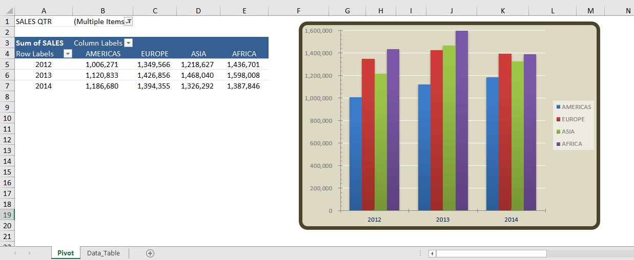
2.5. Pivot Charts
Pivot charts are visual representations of pivot table data. They make it easier to identify trends and patterns.
2.5.1. How to Create a Pivot Chart
- Select the Pivot Table: Click anywhere inside the pivot table.
- Go to the “Analyze” Tab: In the Excel ribbon, find the “PivotTable Analyze” tab (or “Options” tab in older versions).
- Click “PivotChart”: In the “Tools” group, click “PivotChart”.
- Choose a Chart Type: Select the chart type you want to create (e.g., column, line, pie).
- Click “OK”: The pivot chart will appear on your worksheet.
2.5.2. Using Pivot Charts for Comparisons
- Column Charts: Compare values across different categories.
- Line Charts: Show trends over time.
- Bar Charts: Compare values side-by-side for easy comparison.
- Pie Charts: Show proportions of different categories.
3. Step-by-Step Guide: Comparing Two Pivot Tables
Here’s a detailed guide on how to compare two pivot tables for differences, complete with examples and best practices.
3.1. Scenario: Year-over-Year Sales Comparison
Let’s say you want to compare sales data from 2022 and 2023 to see how your company performed year-over-year.
3.1.1. Data Setup
First, ensure your data includes columns for:
- Date: The date of each sale.
- Sales: The amount of each sale.
- Product: The product sold.
- Region: The region where the sale occurred.
3.1.2. Create the First Pivot Table
- Select Your Data: Select the range containing your data.
- Insert Pivot Table: Go to “Insert” > “PivotTable”.
- Choose Location: Select “New Worksheet” or “Existing Worksheet” and click “OK”.
- Add Fields:
- Drag “Date” to the Rows area. Right-click on the date field in the pivot table and select “Group”. Group by “Years”.
- Drag “Sales” to the Values area.
- Rename Columns: Rename the columns for clarity (e.g., “Year” and “Sales”).
3.1.3. Create the Second Pivot Table
Repeat the steps above to create a second pivot table. Ensure it is based on the same data source as the first one.
3.1.4. Compare Using “Difference From”
- Add Sales Field Again: Drag the “Sales” field to the Values area again. You should now have two “Sum of Sales” fields.
- Show Values As: Right-click on the second “Sum of Sales” field and select “Show Values As” > “Difference From”.
- Configure Comparison:
- Base field: Year
- Base item: Previous
- Click “OK”.
Your pivot table now shows the difference in sales between each year and the previous year.
3.1.5. Show Percentage Difference
- Add Sales Field Again: Drag the “Sales” field to the Values area again.
- Show Values As: Right-click on the third “Sum of Sales” field and select “Show Values As” > “% Difference From”.
- Configure Comparison:
- Base field: Year
- Base item: Previous
- Click “OK”.
Now, your pivot table displays both the absolute difference and the percentage difference in sales year-over-year.
3.2. Scenario: Budget vs. Actuals Comparison
Suppose you want to compare your budget against actual expenses to identify variances.
3.2.1. Data Setup
Your data should include columns for:
- Category: Expense categories (e.g., Rent, Salaries, Marketing).
- Budget: The budgeted amount for each category.
- Actual: The actual amount spent for each category.
3.2.2. Create the Pivot Table
- Select Your Data: Select the range containing your data.
- Insert Pivot Table: Go to “Insert” > “PivotTable”.
- Choose Location: Select “New Worksheet” or “Existing Worksheet” and click “OK”.
- Add Fields:
- Drag “Category” to the Rows area.
- Drag “Budget” and “Actual” to the Values area.
3.2.3. Create a Calculated Field for Variance
- Select the Pivot Table: Click anywhere inside the pivot table.
- Go to the “Analyze” Tab: In the Excel ribbon, find the “PivotTable Analyze” tab (or “Options” tab in older versions).
- Click “Fields, Items, & Sets”: In the “Calculations” group, click “Fields, Items, & Sets”.
- Choose “Calculated Field”: Select “Calculated Field” from the dropdown menu.
- Name the Field: Enter “Variance” in the “Name” box.
- Enter the Formula: In the “Formula” box, enter
=Budget - Actual. - Add the Field: Click “Add” to add the calculated field to your pivot table.
- Click “OK”: Close the Calculated Field dialog box.
3.2.4. Create a Calculated Field for Variance Percentage
- Select the Pivot Table: Click anywhere inside the pivot table.
- Go to the “Analyze” Tab: In the Excel ribbon, find the “PivotTable Analyze” tab (or “Options” tab in older versions).
- Click “Fields, Items, & Sets”: In the “Calculations” group, click “Fields, Items, & Sets”.
- Choose “Calculated Field”: Select “Calculated Field” from the dropdown menu.
- Name the Field: Enter “Variance %” in the “Name” box.
- Enter the Formula: In the “Formula” box, enter
=(Budget - Actual) / Budget. - Add the Field: Click “Add” to add the calculated field to your pivot table.
- Click “OK”: Close the Calculated Field dialog box.
Your pivot table now shows the budget, actual expenses, variance, and variance percentage for each category.
3.3. Scenario: Regional Performance Comparison
Let’s say you want to compare sales performance across different regions.
3.3.1. Data Setup
Your data should include columns for:
- Region: The geographic region of the sale.
- Sales: The amount of each sale.
- Product: The product sold.
3.3.2. Create the Pivot Table
- Select Your Data: Select the range containing your data.
- Insert Pivot Table: Go to “Insert” > “PivotTable”.
- Choose Location: Select “New Worksheet” or “Existing Worksheet” and click “OK”.
- Add Fields:
- Drag “Region” to the Rows area.
- Drag “Sales” to the Values area.
3.3.3. Add Slicers for Product and Date
- Select the Pivot Table: Click anywhere inside the pivot table.
- Go to the “Analyze” Tab: In the Excel ribbon, find the “PivotTable Analyze” tab (or “Options” tab in older versions).
- Click “Insert Slicer”: In the “Filter” group, click “Insert Slicer”.
- Choose Fields: Select “Product” and “Date” in the “Insert Slicers” dialog box.
- Click “OK”: The slicers will appear on your worksheet.
3.3.4. Analyze Performance with Slicers
Use the slicers to filter the data and compare sales performance for different products and time periods across regions.
4. Advanced Techniques and Tips
To further enhance your pivot table comparisons, consider these advanced techniques and tips.
4.1. Using Power Pivot for Complex Data
Power Pivot is an Excel add-in that allows you to analyze large and complex datasets from multiple sources. It’s especially useful when your data is spread across multiple tables.
4.1.1. How to Use Power Pivot
- Enable Power Pivot: Go to “File” > “Options” > “Add-Ins”. In the “Manage” dropdown, select “COM Add-ins” and click “Go”. Check the box next to “Microsoft Power Pivot for Excel” and click “OK”.
- Import Data: In the Power Pivot window, click “From Database” or “From Other Sources” to import your data.
- Create Relationships: Create relationships between your tables by dragging fields from one table to another in the Diagram View.
- Create Pivot Table: Click “PivotTable” to create a pivot table based on your Power Pivot data model.
4.1.2. Benefits of Using Power Pivot
- Handles Large Datasets: Power Pivot can handle millions of rows of data, which is more than Excel’s built-in pivot tables can handle.
- Multiple Data Sources: You can combine data from multiple sources, such as Excel files, databases, and text files.
- Complex Relationships: Power Pivot allows you to create complex relationships between tables, enabling more sophisticated analysis.
4.2. DAX Formulas for Advanced Calculations
DAX (Data Analysis Expressions) is a formula language used in Power Pivot. It allows you to create advanced calculations that are not possible with Excel’s built-in formulas.
4.2.1. Examples of DAX Formulas
- Calculate Year-to-Date Sales:
TotalYTD := TOTALYTD(SUM(Sales[Amount]), Dates[Date])- Calculate Moving Average:
MovingAverage :=
AVERAGEX (
    FILTER (
        ALL (Dates[Date]),
        Dates[Date] <= MAX (Dates[Date])
            && Dates[Date]
               >= MAX (Dates[Date]) - 6
    ),
    CALCULATE (SUM (Sales[Amount]))
)
4.3. Conditional Formatting for Visual Cues
Conditional formatting allows you to apply formatting to cells based on their values. This can help you quickly identify important data points.
4.3.1. How to Apply Conditional Formatting
- Select the Data: Select the range of cells you want to format.
- Go to “Conditional Formatting”: In the “Home” tab, click “Conditional Formatting”.
- Choose a Rule Type: Select a rule type (e.g., “Highlight Cells Rules”, “Top/Bottom Rules”, “Data Bars”, “Color Scales”, “Icon Sets”).
- Configure the Rule: Specify the criteria for the formatting (e.g., values greater than a certain number, top 10%, above average).
- Choose a Format: Select the formatting you want to apply (e.g., fill color, font color, icons).
- Click “OK”: The conditional formatting will be applied to your data.
4.3.2. Examples of Conditional Formatting for Comparisons
- Highlight Values Above a Threshold: Highlight sales figures above a certain target.
- Use Color Scales to Show Variance: Use a color scale to show the magnitude of variance between budget and actual expenses.
- Use Icon Sets to Indicate Trends: Use icons to indicate whether sales are increasing, decreasing, or staying the same.
5. Troubleshooting Common Issues
When comparing pivot tables, you might encounter some common issues. Here’s how to troubleshoot them.
5.1. Data Source Issues
- Inconsistent Data: Ensure your data is consistent across all sources. Check for spelling errors, inconsistent formatting, and missing values.
- Incorrect Data Types: Make sure your data types are correct (e.g., numbers are formatted as numbers, dates are formatted as dates).
- Missing Data: Handle missing data appropriately. You can either fill in the missing values or exclude them from your analysis.
5.2. Pivot Table Errors
- #DIV/0! Error: This error occurs when you try to divide by zero. Check your formulas and ensure that the denominator is not zero.
- #REF! Error: This error occurs when a cell reference is invalid. Check your formulas and ensure that all cell references are correct.
- #VALUE! Error: This error occurs when a formula contains an incorrect data type. Check your data types and ensure that they are compatible with your formulas.
5.3. Comparison Problems
- Incorrect Base Field or Item: Double-check that you have selected the correct base field and item when using the “Show Values As” option.
- Incorrect Formula: Review your formulas to ensure that they are calculating the correct values.
- Filtering Issues: Ensure that your filters are applied correctly and that they are not excluding important data.
6. Case Studies: Real-World Examples
Let’s look at some real-world examples of how pivot table comparisons can be used.
6.1. Retail Sales Analysis
A retail company uses pivot tables to compare sales performance across different stores, product categories, and time periods. By using the “Show Values As” option, they can quickly identify which stores are outperforming or underperforming, which product categories are driving the most sales, and how sales trends are changing over time.
6.2. Financial Budgeting
A financial department uses pivot tables to compare budgeted amounts against actual expenses. By creating calculated fields for variance and variance percentage, they can quickly identify areas where spending is exceeding the budget and take corrective action.
6.3. Marketing Campaign Analysis
A marketing team uses pivot tables to analyze the performance of different marketing campaigns. By comparing metrics such as leads, conversions, and ROI, they can determine which campaigns are the most effective and optimize their marketing strategy accordingly.
7. Conclusion: Mastering Pivot Table Comparisons
Comparing pivot tables is a powerful way to gain insights from your data. By mastering Excel’s built-in features, such as the “Show Values As” option, calculated fields, slicers, timelines, and pivot charts, you can easily identify trends, analyze variance, and make data-driven decisions. Whether you’re tracking sales, managing budgets, or analyzing marketing campaigns, pivot tables provide a flexible and intuitive way to summarize and compare your data.
Struggling to compare data effectively? Visit COMPARE.EDU.VN for expert guidance and tools that simplify the comparison process. Our resources help you make informed decisions by providing clear, comprehensive, and actionable insights. Explore our site to learn more about pivot table comparisons and other data analysis techniques. Contact us at 333 Comparison Plaza, Choice City, CA 90210, United States, or Whatsapp: +1 (626) 555-9090. Check out compare.edu.vn today.
8. Frequently Asked Questions (FAQ)
8.1. How Do I Add a Year Column to My Pivot Table?
To add a Year column to your pivot table, start by ensuring your data source has a date column. If it doesn’t, you may need to first insert the dates manually. Then, add a new column adjacent to your data, and label it “Year.” In the first cell of this new column, use a formula like =YEAR(date_cell) where date_cell is the cell reference containing the date. Drag this formula down to fill the rest of the cells in the column with the corresponding years.
Afterward, refresh your pivot table data source to include the newly added Year column. When you open the PivotTable Field List, you should now see the Year field available. You can then add this to the Rows or Columns area of your pivot table layout to start analyzing your data by year.
Remember, this Year column is crucial for performing year-over-year analysis, so having it in your pivot table setup is essential.
8.2. Can Pivot Tables Calculate Percentage Differences Automatically?
Absolutely, pivot tables can automatically calculate percentage differences without you needing to do the math. Once you have your pivot table set up, you can use the “Show Values As” feature to compare two periods. For example, to show the percent difference in sales between two years, you would:
- Add your Sales data to the Values area of the pivot table twice.
- Right-click on the second instance of your Sales data in the pivot table.
- Choose “Show Values As” then select “% Difference From.”
- In the dialog box that appears, select the base field, such as the Year, and choose the specific year or “(previous)” to compare against the previous period.
Your pivot table will now display the percentage differences for you. This is particularly useful for analyzing trends over time, giving you a clear view of growth or decline.
8.3. How Can I Compare Data from Two Different Excel Files?
Comparing data from two different Excel files involves a few steps. First, ensure both files are open in Excel. Then, create pivot tables in each file using the respective data. To compare the data, you can either manually compare the pivot tables side-by-side or consolidate the data into one file.
To consolidate, copy the data from one file and paste it into the other. Ensure that the columns align correctly. Once the data is in one file, create a single pivot table that includes all the data. You can then use filters, slicers, and calculated fields to compare the data from the two original files.
8.4. What Are the Best Chart Types for Comparing Pivot Table Data?
The best chart types for comparing pivot table data depend on what you want to emphasize. Column charts and bar charts are excellent for comparing values across different categories. Line charts are ideal for showing trends over time. Pie charts are useful for showing proportions of different categories.
For more complex comparisons, consider using scatter plots or bubble charts to show relationships between multiple variables. Experiment with different chart types to find the one that best communicates your data.
8.5. How Do I Filter Data in a Pivot Table?
Filtering data in a pivot table is straightforward. You can use the filter arrows next to the row and column labels to select specific items to include in your analysis. Additionally, you can use slicers and timelines for more interactive filtering.
To add a slicer, select the pivot table and go to the “Analyze” tab. Click “Insert Slicer” and choose the fields you want to use as filters. For date fields, you can insert a timeline. Slicers and timelines provide a visual way to filter your data and compare different subsets.
8.6. Can I Use Formulas in Pivot Tables?
Yes, you can use formulas in pivot tables by creating calculated fields. To create a calculated field, select the pivot table and go to the “Analyze” tab. Click “Fields, Items, & Sets” and choose “Calculated Field.” Enter a name for your field and a formula that uses existing fields in the pivot table.
Calculated fields allow you to create custom metrics and comparisons within your pivot table. For example, you can create a calculated field to calculate profit margin, growth rate, or variance.
8.7. How Do I Group Data in a Pivot Table?
Grouping data in a pivot table allows you to combine related items into categories. To group data, right-click on a row or column label and select “Group.” You can group items manually or automatically based on numerical or date ranges.
For example, you can group dates by year, quarter, or month. You can also group numerical values into ranges, such as age groups or income brackets. Grouping data makes it easier to analyze trends and patterns in your data.
8.8. How Do I Refresh a Pivot Table?
To refresh a pivot table, right-click anywhere inside the pivot table and select “Refresh.” This will update the pivot table with any changes made to the data source. You can also refresh all pivot tables in a workbook by going to the “Data” tab and clicking “Refresh All.”
It’s important to refresh your pivot tables regularly to ensure that they are displaying the most up-to-date information. You can also set up automatic refresh options in the pivot table settings.
8.9. What Is the Difference Between a Pivot Table and a Regular Table?
A regular table is a simple grid of rows and columns that stores data. A pivot table, on the other hand, is a dynamic tool that summarizes and analyzes data from a regular table.
Pivot tables allow you to rearrange and recalculate data to see different summaries without altering the original data source. They provide a flexible way to explore your data and identify trends and patterns. Regular tables are primarily used for data storage, while pivot tables are used for data analysis.
8.10. How Can I Share My Pivot Table with Others?
You can share your pivot table with others by saving the Excel file and sending it to them. If you want to share a static view of the data, you can copy the pivot table and paste it as values into another worksheet or document.
For more interactive sharing, consider using Excel Online or other collaboration tools that allow multiple users to view and interact with the pivot table simultaneously. Always ensure that the data source is accessible to the recipients if they need to refresh the pivot table.