How Do I Compare Two Lists In Excel For Differences?

Comparing two lists in Excel for differences is achievable through various methods, allowing you to identify unique entries efficiently. At COMPARE.EDU.VN, we provide comprehensive guides to help you master these techniques. By employing formulas, conditional formatting, or specialized tools, you can easily pinpoint discrepancies between datasets, optimizing data analysis and decision-making. Enhance your Excel skills and streamline your comparative tasks with our expert insights.

1. Understanding the Need for Comparing Lists in Excel

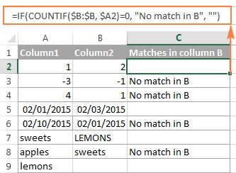
Comparing two lists in Excel to find differences is a common requirement across various fields. Whether you’re managing inventory, tracking sales data, or ensuring data accuracy, the ability to quickly identify discrepancies can save time and reduce errors. Excel offers several built-in functions and features that can help you accomplish this task, each with its own advantages and use cases. Understanding these tools will empower you to choose the most efficient method for your specific needs.
Comparing two lists in excel using COUNTIF function for identifying differences

1.1. Why Compare Lists in Excel?

The need to compare lists in Excel arises in numerous situations, such as:

• Data Validation: Ensuring that data entered into a system matches a master list.
• Inventory Management: Identifying discrepancies between expected and actual stock levels.
• Sales Analysis: Comparing sales data from different periods to identify growth or decline.
• Customer Relationship Management (CRM): Checking for duplicate customer entries.
• Project Management: Tracking task completion against a planned schedule.

1.2. Common Challenges in Comparing Lists

While Excel provides tools for comparing lists, users often face challenges such as:

• Large Datasets: Manually comparing large lists is time-consuming and prone to error.
• Data Formatting: Inconsistent formatting (e.g., different date formats or text casing) can lead to inaccurate comparisons.
• Complex Criteria: Identifying differences based on multiple criteria can be challenging to implement.
• Dynamic Lists: When lists are frequently updated, maintaining accurate comparisons can be difficult.

1.3. Overview of Comparison Methods

Excel offers several methods for comparing lists to find differences, each suited to different scenarios:

• IF and COUNTIF Functions: These functions can be used to identify entries in one list that do not appear in another.
• VLOOKUP and MATCH Functions: These functions are useful for finding matches and identifying missing entries between two lists.
• Conditional Formatting: This feature allows you to visually highlight differences between lists.
• Advanced Filter: This tool can be used to filter out matching entries, leaving only the differences.
• Specialized Add-ins: Third-party add-ins, such as those offered by Ablebits, provide more advanced comparison capabilities.

2. Using IF and COUNTIF Functions for List Comparison

The IF and COUNTIF functions are powerful tools for comparing two lists in Excel, especially when you need to identify items present in one list but not in another. This method is particularly useful for simple comparisons and can be easily adapted to various scenarios.

2.1. Basic Syntax and Functionality

• COUNTIF Function: The COUNTIF function counts the number of cells within a range that meet a given criterion. Its syntax is:

  =COUNTIF(range, criteria)

  • range: The range of cells to be evaluated.
  • criteria: The condition that determines which cells will be counted.

• IF Function: The IF function returns one value if a condition is true and another value if the condition is false. Its syntax is:

  =IF(logical_test, value_if_true, value_if_false)

  • logical_test: The condition to be evaluated.
  • value_if_true: The value to return if the condition is true.
  • value_if_false: The value to return if the condition is false.

2.2. Step-by-Step Guide

To compare two lists using IF and COUNTIF, follow these steps:

1. Prepare Your Data: Ensure your two lists are in separate columns in the same worksheet. For example, List 1 might be in column A, and List 2 in column B.

2. Apply the COUNTIF Function: In a new column (e.g., column C), use the COUNTIF function to check if each item in List 1 exists in List 2. Enter the following formula in cell C2 and drag it down to the last item in List 1:

   =COUNTIF($B:$B, A2)

   This formula counts how many times the value in cell A2 appears in column B.

3. Interpret the Results:

   • If the result is 0, the item in List 1 does not appear in List 2.
   • If the result is greater than 0, the item in List 1 appears in List 2 at least once.

4. Use the IF Function to Label Differences: In another new column (e.g., column D), use the IF function to label the differences based on the results from the COUNTIF function. Enter the following formula in cell D2 and drag it down:

   =IF(COUNTIF($B:$B, A2)=0, "Not in List 2", "")

   This formula checks if the COUNTIF result is 0. If it is, it labels the item as “Not in List 2”; otherwise, it leaves the cell blank.

2.3. Example Scenario

Consider two lists: a list of products in stock (List 1) and a list of products sold (List 2). You want to identify which products in stock have not been sold.

• List 1 (Column A): Apple, Banana, Orange, Grape
• List 2 (Column B): Banana, Orange, Kiwi

1. Apply COUNTIF: In cell C2, enter =COUNTIF($B:$B, A2). Drag the formula down to C5. The results will be:
   • C2 (Apple): 0
   • C3 (Banana): 1
   • C4 (Orange): 1
   • C5 (Grape): 0
2. Apply IF: In cell D2, enter =IF(COUNTIF($B:$B, A2)=0, "Not in List 2", ""). Drag the formula down to D5. The results will be:
   • D2 (Apple): Not in List 2
   • D3 (Banana):
   • D4 (Orange):
   • D5 (Grape): Not in List 2

This shows that Apple and Grape are in stock but have not been sold.

2.4. Advantages and Limitations

• Advantages:
  • Simple to implement.
  • No need for advanced Excel skills.
  • Works well for small to medium-sized lists.
• Limitations:
  • Can be slow for very large lists.
  • Only identifies whether an item is present or absent, not the extent of differences.
  • Requires additional columns for the formulas.

3. Utilizing VLOOKUP and MATCH Functions for Advanced Comparisons

For more advanced list comparisons, Excel’s VLOOKUP and MATCH functions offer powerful capabilities. These functions allow you to not only identify differences but also retrieve related information from one list to another.

3.1. Understanding VLOOKUP and MATCH

• VLOOKUP Function: The VLOOKUP function searches for a value in the first column of a range and returns a value in the same row from a specified column. Its syntax is:

  =VLOOKUP(lookup_value, table_array, col_index_num, [range_lookup])

  • lookup_value: The value to search for.
  • table_array: The range of cells to search in.
  • col_index_num: The column number in the range from which to return a value.
  • [range_lookup]: An optional argument that specifies whether to find an exact or approximate match. Use FALSE for exact matches.

• MATCH Function: The MATCH function searches for a specified item in a range of cells and returns the relative position of that item in the range. Its syntax is:

  =MATCH(lookup_value, lookup_array, [match_type])

  • lookup_value: The value to search for.
  • lookup_array: The range of cells to search in.
  • [match_type]: An optional argument that specifies the type of match. Use 0 for exact matches.

3.2. Step-by-Step Guide Using VLOOKUP

To compare two lists using VLOOKUP, follow these steps:

1. Prepare Your Data: Ensure your two lists are in separate columns in the same worksheet. For example, List 1 (the list you want to check for differences) is in column A, and List 2 (the reference list) is in column B.

2. Apply the VLOOKUP Function: In a new column (e.g., column C), use the VLOOKUP function to search for each item in List 1 within List 2. Enter the following formula in cell C2 and drag it down to the last item in List 1:

   =VLOOKUP(A2, $B:$B, 1, FALSE)

   This formula searches for the value in cell A2 within column B. The 1 indicates that it should return the value from the first column of the found range (which is the value itself), and FALSE ensures an exact match.

3. Interpret the Results:

   • If the VLOOKUP function finds a match, it returns the matched value.
   • If the VLOOKUP function does not find a match, it returns the #N/A error.

4. Use the ISNA Function to Identify Differences: In another new column (e.g., column D), use the ISNA function to identify the #N/A errors, indicating the differences. Enter the following formula in cell D2 and drag it down:

   =IF(ISNA(VLOOKUP(A2, $B:$B, 1, FALSE)), "Not in List 2", "")

   This formula checks if the VLOOKUP result is #N/A. If it is, it labels the item as “Not in List 2”; otherwise, it leaves the cell blank.

3.3. Step-by-Step Guide Using MATCH

To compare two lists using MATCH, follow these steps:

1. Prepare Your Data: Ensure your two lists are in separate columns.

2. Apply the MATCH Function: In a new column (e.g., column C), use the MATCH function to find the position of each item in List 1 within List 2. Enter the following formula in cell C2 and drag it down:

   =MATCH(A2, $B:$B, 0)

   This formula searches for the value in cell A2 within column B. The 0 ensures an exact match.

3. Interpret the Results:

   • If the MATCH function finds a match, it returns the position of the matched value in List 2.
   • If the MATCH function does not find a match, it returns the #N/A error.

4. Use the ISNA Function to Identify Differences: In another new column (e.g., column D), use the ISNA function to identify the #N/A errors, indicating the differences. Enter the following formula in cell D2 and drag it down:

   =IF(ISNA(MATCH(A2, $B:$B, 0)), "Not in List 2", "")

   This formula checks if the MATCH result is #N/A. If it is, it labels the item as “Not in List 2”; otherwise, it leaves the cell blank.

3.4. Example Scenario

Consider two lists: a list of employee IDs (List 1) and a list of active employee IDs (List 2). You want to identify which employees are no longer active.

• List 1 (Column A): 101, 102, 103, 104
• List 2 (Column B): 102, 103, 105

1. Apply VLOOKUP: In cell C2, enter =VLOOKUP(A2, $B:$B, 1, FALSE). Drag the formula down to C5. The results will be:
   • C2 (101): #N/A
   • C3 (102): 102
   • C4 (103): 103
   • C5 (104): #N/A
2. Apply ISNA: In cell D2, enter =IF(ISNA(VLOOKUP(A2, $B:$B, 1, FALSE)), "Not in List 2", ""). Drag the formula down to D5. The results will be:
   • D2 (101): Not in List 2
   • D3 (102):
   • D4 (103):
   • D5 (104): Not in List 2

This shows that employee IDs 101 and 104 are not in the active employee list.

3.5. Advantages and Limitations

• Advantages:
  • More efficient for medium to large-sized lists.
  • Can retrieve additional information associated with the matched values.
  • Provides more detailed results than IF and COUNTIF.
• Limitations:
  • Requires a good understanding of VLOOKUP and MATCH syntax.
  • Can be slower than COUNTIF for very simple comparisons.
  • Returns errors when no match is found, which need to be handled using ISNA or IFERROR.

4. Visualizing Differences with Conditional Formatting

Conditional formatting in Excel is an effective way to highlight differences between two lists visually. This method allows you to quickly identify discrepancies without having to manually compare each entry.

4.1. Basic Principles of Conditional Formatting

Conditional formatting allows you to apply formatting (e.g., colors, fonts, icons) to cells based on specific criteria. To compare two lists, you can use conditional formatting rules to highlight items that are unique to one list or common to both.

4.2. Step-by-Step Guide to Highlight Unique Entries

To highlight unique entries in two lists using conditional formatting, follow these steps:

1. Prepare Your Data: Ensure your two lists are in separate columns in the same worksheet. For example, List 1 is in column A, and List 2 is in column B.

2. Select List 1: Select all the cells in List 1 (e.g., A2:A10).

3. Open Conditional Formatting: Go to the “Home” tab, click on “Conditional Formatting,” and select “New Rule.”

4. Create a New Rule: In the “New Formatting Rule” dialog box, select “Use a formula to determine which cells to format.”

5. Enter the Formula: Enter the following formula in the formula box:

   =COUNTIF($B:$B, A2)=0

   This formula checks if the value in cell A2 does not exist in column B.

6. Set the Formatting: Click the “Format” button, go to the “Fill” tab, and choose a color to highlight the unique entries (e.g., red). Click “OK” twice to close the dialog boxes.

7. Repeat for List 2: Select all the cells in List 2 (e.g., B2:B10) and repeat steps 3-6, but use the following formula:

   =COUNTIF($A:$A, B2)=0

   This formula checks if the value in cell B2 does not exist in column A. Choose a different color to highlight the unique entries in List 2 (e.g., blue).

4.3. Step-by-Step Guide to Highlight Matching Entries

To highlight matching entries in two lists using conditional formatting, follow these steps:

1. Prepare Your Data: Ensure your two lists are in separate columns.

2. Select List 1: Select all the cells in List 1.

3. Open Conditional Formatting: Go to the “Home” tab, click on “Conditional Formatting,” and select “New Rule.”

4. Create a New Rule: In the “New Formatting Rule” dialog box, select “Use a formula to determine which cells to format.”

5. Enter the Formula: Enter the following formula in the formula box:

   =COUNTIF($B:$B, A2)>0

   This formula checks if the value in cell A2 exists in column B.

6. Set the Formatting: Click the “Format” button, go to the “Fill” tab, and choose a color to highlight the matching entries (e.g., green). Click “OK” twice to close the dialog boxes.

7. Repeat for List 2: Select all the cells in List 2 and repeat steps 3-6, but use the following formula:

   =COUNTIF($A:$A, B2)>0

   This formula checks if the value in cell B2 exists in column A. Choose the same color to highlight the matching entries in List 2 (e.g., green).

4.4. Example Scenario

Consider two lists: a list of registered users (List 1) and a list of newsletter subscribers (List 2). You want to visually identify which registered users are not subscribed to the newsletter and vice versa.

• List 1 (Column A): John, Jane, Mike, Emily
• List 2 (Column B): Jane, Emily, David

1. Highlight Unique Entries in List 1: Using the formula =COUNTIF($B:$B, A2)=0, highlight John and Mike in red.
2. Highlight Unique Entries in List 2: Using the formula =COUNTIF($A:$A, B2)=0, highlight David in blue.
3. Highlight Matching Entries: Using the formula =COUNTIF($B:$B, A2)>0 and =COUNTIF($A:$A, B2)>0, highlight Jane and Emily in green in both lists.

4.5. Advantages and Limitations

• Advantages:
  • Provides a quick visual overview of differences and matches.
  • Easy to set up and customize.
  • No need for additional columns.
• Limitations:
  • Can be difficult to interpret with very large lists.
  • Does not provide detailed information about the differences.
  • Formatting can slow down Excel with complex rules and large datasets.

5. Advanced Filtering for Efficient List Comparison

Excel’s Advanced Filter feature offers a powerful way to extract differences between two lists. Unlike basic filtering, Advanced Filter allows you to use complex criteria and copy the results to another location, making it ideal for comparing lists and identifying unique entries.

5.1. Understanding Advanced Filter

Advanced Filter allows you to filter a list based on complex criteria and extract the filtered data to another location. This feature is particularly useful when you need to compare two lists and identify the entries that are present in one list but not in the other.

5.2. Step-by-Step Guide

To compare two lists using Advanced Filter, follow these steps:

1. Prepare Your Data: Ensure your two lists are in separate columns in the same worksheet. Add a header row above each list (e.g., “List1” above column A and “List2” above column B).

2. Create a Criteria Range: In a separate area of your worksheet, create a criteria range. This range consists of a header row and a row containing the criteria for filtering.

   • In the header row, enter the header of the list you want to filter (e.g., “List1”).

   • In the row below the header, enter the following formula:

     =COUNTIF(List2,List1)=0

     Replace List2 with the range of cells containing your second list (e.g., $B$2:$B$10) and List1 with the cell containing the first item in your first list (e.g., A2).

3. Open Advanced Filter: Go to the “Data” tab and click on “Advanced” in the “Sort & Filter” group.

4. Set the Filter Options: In the “Advanced Filter” dialog box, configure the following settings:

   • Action: Choose “Copy to another location.”
   • List range: Select the range of cells containing your first list, including the header (e.g., $A$1:$A$10).
   • Criteria range: Select the range of cells containing your criteria range, including the header and the formula (e.g., $D$1:$D$2).
   • Copy to: Select a cell where you want the filtered results to be copied (e.g., E1).
   • Check the “Unique records only” box if you only want to extract unique entries.

5. Apply the Filter: Click “OK” to apply the filter. The unique entries from List 1 that do not appear in List 2 will be copied to the specified location.

5.3. Example Scenario

Consider two lists: a list of attendees for an event (List 1) and a list of registered participants (List 2). You want to identify which attendees did not register.

• List 1 (Column A): John, Jane, Mike, Emily
• List 2 (Column B): Jane, Emily, David

1. Create a Criteria Range:
   • In cell D1, enter “List1.”
   • In cell D2, enter the formula =COUNTIF($B$2:$B$4, A2)=0.
2. Open Advanced Filter: Go to “Data” > “Advanced.”
3. Set the Filter Options:
   • List range: $A$1:$A$5
   • Criteria range: $D$1:$D$2
   • Copy to: E1
4. Apply the Filter: Click “OK.” The results in column E will be:
   • John
   • Mike

This shows that John and Mike attended the event but did not register.

5.4. Advantages and Limitations

• Advantages:
  • Can handle complex criteria for filtering.
  • Extracts the filtered data to another location, preserving the original lists.
  • Allows for unique records only extraction.
• Limitations:
  • Requires creating a criteria range with formulas.
  • Can be complex to set up for users unfamiliar with advanced filtering.
  • The criteria range must be set up correctly for the filter to work accurately.

6. Using Specialized Add-ins for Comprehensive Comparisons

While Excel’s built-in functions and features are useful for comparing lists, specialized add-ins offer more comprehensive capabilities, particularly for complex comparisons and large datasets. These add-ins often provide intuitive interfaces and advanced options that streamline the comparison process.

6.1. Overview of Specialized Add-ins

Several Excel add-ins are designed to enhance list comparison capabilities. These add-ins typically offer features such as:

• Multi-Column Comparison: Comparing lists based on multiple columns or criteria.
• Fuzzy Matching: Identifying similar but not identical entries.
• Data Merging: Merging data from two lists based on matching criteria.
• Change Tracking: Identifying changes made to lists over time.
• Reporting: Generating detailed reports of the comparison results.

6.2. Example: Ablebits Ultimate Suite

One popular add-in is Ablebits Ultimate Suite, which includes a “Compare Two Tables” tool. This tool simplifies the process of comparing lists and offers several advanced features.

6.2.1. Step-by-Step Guide Using Ablebits Ultimate Suite

To compare two lists using Ablebits Ultimate Suite, follow these steps:

1. Install Ablebits Ultimate Suite: Download and install the Ablebits Ultimate Suite add-in for Excel from the Ablebits website.
2. Open the Compare Tables Tool: Go to the “Ablebits Data” tab in Excel and click on “Compare Tables.”
3. Select the Lists: In the “Compare Tables” dialog box, select the two lists you want to compare. You can select the lists by dragging your mouse over the ranges or by entering the cell ranges manually.
4. Choose the Comparison Type: Select the type of comparison you want to perform:
   • Duplicate values: Identifies items that exist in both lists.
   • Unique values: Identifies items that are present in one list but not in the other.
5. Select the Columns for Comparison: Choose the columns you want to use for comparison. You can compare based on one or more columns.
6. Choose the Output Options: Select how you want to handle the results:
   • Highlight with color: Highlights the matches or differences in the selected color.
   • Identify in the Status column: Inserts a “Status” column with labels such as “Duplicate” or “Unique.”
7. Run the Comparison: Click “Finish” to run the comparison. The results will be displayed according to the output options you selected.

6.2.2. Example Scenario

Consider two lists: a list of products in a catalog (List 1) and a list of products sold in a store (List 2). You want to identify which products in the catalog are not being sold in the store.

• List 1 (Catalog): Apple, Banana, Orange, Grape
• List 2 (Sold): Banana, Orange, Kiwi

1. Open Compare Tables: Go to “Ablebits Data” > “Compare Tables.”
2. Select the Lists: Select the range containing List 1 (e.g., $A$1:$A$5) and the range containing List 2 (e.g., $B$1:$B$4).
3. Choose the Comparison Type: Select “Unique values” to find items in List 1 that are not in List 2.
4. Select the Columns for Comparison: Choose the columns containing the product names.
5. Choose the Output Options: Select “Highlight with color” and choose a color (e.g., red) to highlight the unique entries.
6. Run the Comparison: Click “Finish.” The results will be:
   • Apple and Grape in List 1 will be highlighted in red, indicating that they are not being sold in the store.

6.3. Advantages and Limitations

• Advantages:
  • Provides a comprehensive set of features for complex list comparisons.
  • Offers an intuitive interface that simplifies the comparison process.
  • Can handle large datasets efficiently.
  • Provides detailed reports of the comparison results.
• Limitations:
  • Requires purchasing and installing a third-party add-in.
  • May have a learning curve for users unfamiliar with the add-in.
  • Some add-ins may be expensive.

7. Practical Examples and Use Cases

To further illustrate the methods for comparing two lists in Excel, let’s explore some practical examples and use cases across different scenarios.

7.1. Inventory Management

Scenario: A retail store needs to compare its physical inventory count with its inventory management system to identify discrepancies.

• List 1 (Column A): List of items in the inventory management system (e.g., product ID, name, quantity).
• List 2 (Column B): List of items counted during the physical inventory count.

Methods to Use:

1. IF and COUNTIF: Use COUNTIF to check if each item in List 1 exists in List 2. Then, use IF to label the differences (e.g., “Missing in Physical Count”).
2. VLOOKUP: Use VLOOKUP to search for each item in List 1 within List 2 and retrieve the quantity. If #N/A is returned, the item is missing in the physical count.
3. Conditional Formatting: Highlight items that are unique to either list to visually identify discrepancies.
4. Specialized Add-ins: Use Ablebits Ultimate Suite to compare the lists and generate a report of the differences, including missing items and quantity discrepancies.

7.2. Customer Relationship Management (CRM)

Scenario: A company wants to identify duplicate customer entries in its CRM database.

• List 1 (Column A): List of customer names and email addresses in the CRM database.
• List 2 (Column B): Same as List 1.

Methods to Use:

1. COUNTIF: Use COUNTIF to check if each customer entry appears more than once in the list. If the count is greater than 1, it’s a duplicate.
2. Conditional Formatting: Highlight duplicate entries using conditional formatting to visually identify them.
3. Advanced Filter: Filter the list to show only unique entries and compare it with the original list to identify duplicates.
4. Specialized Add-ins: Use an add-in to compare the lists based on multiple columns (e.g., name, email, phone number) and identify potential duplicates.

7.3. Sales Analysis

Scenario: A sales manager wants to compare sales data from two different months to identify growth and decline in sales.

• List 1 (Column A): List of products sold in January with corresponding sales figures.
• List 2 (Column B): List of products sold in February with corresponding sales figures.

Methods to Use:

1. VLOOKUP: Use VLOOKUP to search for each product in List 1 within List 2 and retrieve the sales figures. Calculate the difference between the January and February sales figures to identify growth and decline.
2. Conditional Formatting: Highlight products with significant growth or decline using conditional formatting.
3. Specialized Add-ins: Use an add-in to compare the lists and generate a report showing the sales growth and decline for each product.

7.4. Project Management

Scenario: A project manager wants to compare the planned task list with the completed task list to identify tasks that are overdue.

• List 1 (Column A): List of planned tasks with due dates.
• List 2 (Column B): List of completed tasks with completion dates.

Methods to Use:

1. VLOOKUP: Use VLOOKUP to search for each task in List 1 within List 2. If #N/A is returned, the task is overdue.
2. IF and TODAY: Use IF and TODAY functions to check if the due date for each task is in the past and if the task is not in the completed task list.
3. Conditional Formatting: Highlight overdue tasks using conditional formatting.

8. Tips and Best Practices for Accurate Comparisons

To ensure accurate and efficient list comparisons in Excel, consider the following tips and best practices:

8.1. Data Cleaning and Preparation

• Consistency: Ensure that the data in both lists is consistent in terms of formatting, spelling, and casing.
• Remove Duplicates: Remove any duplicate entries within each list before comparing them.
• Standardize Formats: Standardize date formats, number formats, and text casing to avoid false negatives.
• Trim Spaces: Remove leading and trailing spaces from text entries using the TRIM function.

8.2. Choosing the Right Method

• Consider List Size: For small to medium-sized lists, IF and COUNTIF functions may be sufficient. For larger lists, VLOOKUP and specialized add-ins are more efficient.
• Complexity of Criteria: If you need to compare based on multiple criteria, consider using advanced filtering or specialized add-ins.
• Required Output: If you need a quick visual overview, conditional formatting is a good choice. If you need detailed reports, specialized add-ins are more suitable.

8.3. Formula Optimization

• Use Absolute References: Use absolute references (e.g., $B$2:$B$10) in formulas to prevent them from changing when copied to other cells.
• Avoid Entire Column References: Avoid using entire column references (e.g., $B:$B) in formulas, as they can slow down Excel. Instead, use specific ranges.
• Use Named Ranges: Use named ranges to make formulas more readable and easier to maintain.

8.4. Testing and Validation

• Test Formulas: Test formulas on a small subset of the data to ensure they are working correctly.
• Validate Results: Validate the comparison results by manually checking a sample of the data.
• Error Handling: Use error handling functions (e.g., IFERROR) to handle errors gracefully and provide meaningful messages.

8.5. Documentation and Collaboration

• Document Steps: Document the steps you took to compare the lists, including the methods used, formulas, and criteria.
• Share Workbooks: Share workbooks with colleagues and provide clear instructions on how to interpret the results.
• Use Comments: Use comments to explain complex formulas and conditional formatting rules.

9. Conclusion: Making Informed Decisions with Excel Comparisons

Comparing two lists in Excel to find differences is a fundamental skill that empowers you to make informed decisions based on accurate data analysis. Whether you are managing inventory, analyzing sales trends, or maintaining customer databases, the ability to quickly identify discrepancies is crucial. Excel offers a range of tools and techniques to accomplish this task, from basic functions like IF and COUNTIF to more advanced features like VLOOKUP, conditional formatting, and specialized add-ins.

By mastering these methods, you can streamline your data analysis processes, reduce errors, and gain valuable insights from your data. Each method has its advantages and limitations, so it’s important to choose the one that best suits your specific needs and data complexity.

At COMPARE.EDU.VN, we are committed to providing you with the knowledge and resources you need to excel in data analysis. Explore our website for more detailed guides, tutorials, and practical examples to enhance your Excel skills and make data-driven decisions with confidence.

Ready to take your Excel skills to the next level? Visit COMPARE.EDU.VN today and discover how our comprehensive resources can help you master list comparisons and other essential data analysis techniques.
Our team is available to assist you. Contact us at:
Address: 333 Comparison Plaza, Choice City, CA 90210, United States
Whatsapp: +1 (626) 555-9090
Website: compare.edu.vn

10. Frequently Asked Questions (FAQ)

1. How do I compare two lists in Excel to find differences?

You can use functions like IF and COUNTIF, VLOOKUP, conditional formatting, advanced filtering, or specialized add-ins like Ablebits Ultimate Suite. The best method depends on the size and complexity of your lists.

2. Can I compare two lists in different worksheets or workbooks?

Yes, you can compare lists in different worksheets or workbooks by referencing the correct ranges in your formulas or by using specialized add-ins that support cross-workbook comparisons.

3. How do I highlight the differences between two lists in Excel?

Use conditional formatting with formulas like =COUNTIF($B:$B, A2)=0 to highlight unique entries or =COUNTIF($B:$B, A2)>0