How Do I Compare Columns In Excel? A Comprehensive Guide

Comparing columns in Excel is essential for data analysis, verification, and identifying discrepancies. At COMPARE.EDU.VN, we offer a complete guide that simplifies the process of comparing columns in Excel, helping you identify matches, mismatches, and unique entries efficiently. Whether you need to highlight differences, find duplicates, or perform complex data validation, our solutions empower you to make informed decisions quickly. Use our step-by-step tutorials to master Excel comparisons, enhancing your data handling capabilities with functions like conditional formatting, the EXACT function, and VLOOKUP.

1. Why Comparing Columns In Excel Is Essential

Excel is widely used for data storage, manipulation, and reporting. The ability to compare two columns is especially valuable for data analysts. This comparison allows them to make informed decisions based on the data present in the columns. Whether the columns are in the same spreadsheet or different ones, manual comparison can be a painstaking and time-consuming task. If data goes missing, it could take hours or even days to complete the process.

Comparing two columns in Excel is crucial for determining whether the cells contain data. Excel displays results as TRUE/FALSE, Match/Not Match, or custom messages.

2. How to Compare Two Columns In Excel: Overview

When you have data in two columns, tables, or spreadsheets, comparing them can help reveal missing or present data in both. Comparisons can take different forms based on your specific needs. Here are several methods you can use:

Highlighting unique or duplicate values in each column using functions.
Displaying unique or duplicate cells using conditional formatting or formulas.
Performing row-by-row comparisons.
Using LOOKUP formulas.

3. Comparing Two Columns Using The Equals Operator

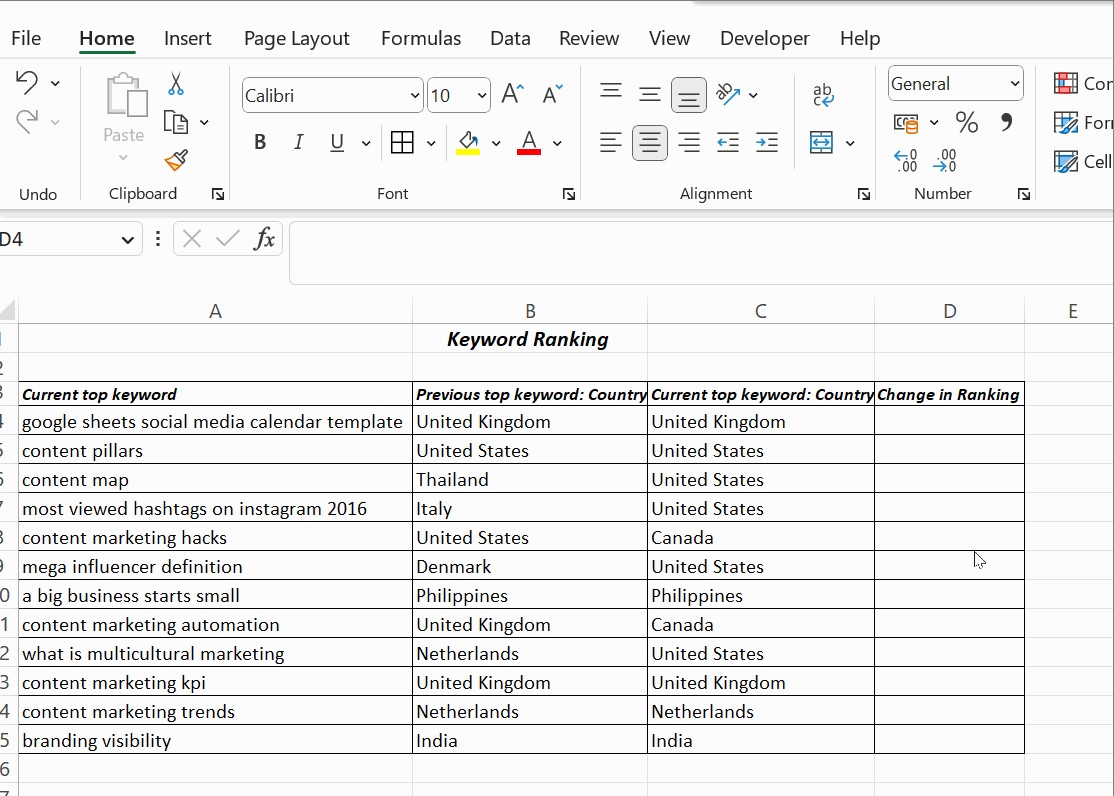
You can compare two columns row by row and find matching data by displaying the result as Match or Not Match. The formula used is =column1=column2. Excel returns TRUE if there is a match and FALSE if there is a mismatch.

For example, in cell D4, you can insert the formula =B4=C4 and press Enter. Then, drag this formula down to the end of the table. The formula returns TRUE if the values in the compared columns are the same and FALSE if the values differ. This is a simple yet effective method for identifying identical entries in two columns.

4. Using The IF Condition to Compare Two Columns

You can also use the IF condition to compare two columns in Excel. The formula to compare two columns is =IF(B4=C4,"Yes"," "). This formula returns Yes for rows with matching values, and the remaining rows are left blank.

4.1. Identifying Mismatching Values with IF Condition

The same formula can also be used to identify and return mismatching values. You need to include an additional argument, No, when the IF condition proves false. The formula is =IF(B4=C4,"Yes","No"). This will display “Yes” for matches and “No” for mismatches, making it easy to spot discrepancies.

4.2. Comparing for Differences

To compare two columns for differences, replace the equals sign with the non-equality sign (<>). The formula is =IF(A2<>B2,"Match","Not a Match"). This formula will return “Match” if the values in the two columns are different and “Not a Match” if they are the same. This is particularly useful when you need to quickly identify any deviations between two sets of data.

5. Case-Sensitive Comparison Using The EXACT() Function

In some cases, you might need to ensure that the comparison is case-sensitive. The standard IF() function does not differentiate between uppercase and lowercase letters.

For example, the IF() function might return Yes when comparing “Netherlands” and “netherlands.” If you need the capitalization to be identical, use the EXACT() function along with IF().

The EXACT() function compares two text strings and returns TRUE only if they are exactly the same, including capitalization.

The syntax for the EXACT() function is =EXACT(text1,text2). It takes two arguments, text1 and text2, both of which are required.

5.1. Implementing Case-Sensitive Comparison

To make the IF condition case-sensitive, use the formula =IF(EXACT(B4,C4), "Match", "Mismatched").

This formula first executes the inner EXACT() function and then returns the result to the outer IF function. The EXACT() function returns TRUE only if the text in both cells is identical, including capitalization. If it returns FALSE, the IF function displays “Mismatched.” This ensures a precise, case-sensitive comparison.

6. Highlighting Differences Using Conditional Formatting

Conditional formatting is another method for comparing two columns in Excel, allowing you to highlight unique or duplicate values.

6.1. Finding Duplicate Values

Select the columns: Select the columns you want to compare.
Open Conditional Formatting: Click Home, then Conditional Formatting in the Styles group.
Highlight Cell Rules: Select Highlight Cell Rules, then Duplicate Values.

This opens a dialog box where you can choose the formatting to apply to duplicate values.
Choose Formatting: Select Duplicate from the drop-down menu.
Customize the Highlight: Choose a formatting option, such as filling with a color, changing the text color, or changing the cell border. You can also select Custom Format to choose a specific color or style.

Click OK to apply the formatting. Excel will highlight all duplicate values in the selected columns, making them easy to identify.

6.2. Highlighting Unique Values

To highlight unique values (i.e., values that appear only in one of the columns):

Select the columns: As before, select the columns you want to compare.
Open Conditional Formatting: Click Home, then Conditional Formatting.
Highlight Cell Rules: Select Highlight Cell Rules, then Duplicate Values.
Choose Unique: In the dialog box, select Unique from the drop-down menu.
Customize the Highlight: Choose a formatting option to highlight the unique values.

Click OK. Excel will now highlight the unique values in the selected columns, allowing you to quickly see which data is not repeated.

6.3. Clearing Conditional Formatting

If you want to remove the conditional formatting:

Open Conditional Formatting: Click Conditional Formatting.
Clear Rules: Select Clear Rules, then Clear Rules from Selected Cells.

Using conditional formatting is beneficial when you want a visual representation of matching or different data without adding a third column to display the results. It is particularly useful for smaller tables where quick visual identification is sufficient.

7. Using Lookup Functions To Compare Columns

Lookup functions can also be used to compare two columns in Excel. These functions search for a value in a row or column and return a corresponding value from another row or column. Common lookup functions include HLOOKUP, VLOOKUP, and XLOOKUP.

7.1. VLOOKUP Function

The VLOOKUP function is particularly useful for comparing columns. The formula is structured as follows:

VLOOKUP(lookup_value, table_array, col_index_num, [range_lookup])

lookup_value: The value you want to search for.
table_array: The range of cells where you want to search.
col_index_num: The column number in the table_array from which to return a value.
[range_lookup]: Optional. TRUE for approximate match, FALSE for exact match.

7.2. Example Using VLOOKUP

Suppose Column A contains a list of keywords, and Column B contains a list of parent keywords. You want to compare Column A with Column B and return the matching parent keywords in Column C.

Enter the Formula: In cell C4, enter the formula =VLOOKUP(A4, $B$4:$B$15, 1, FALSE).
Drag the Cell: Drag the cell down to apply the formula to all cells below C4.

In this formula:

A4 is the lookup value (the keyword you are searching for).
$B$4:$B$15 is the table array (the range of cells containing the parent keywords). The $ symbol creates an absolute reference, ensuring the range does not change when you drag the formula.
1 is the col_index_num, indicating that you want to return the value from the first column of the table_array (which is Column B).
FALSE specifies that you want an exact match.

The VLOOKUP function searches for the value in A4 within the range B4:B15. If it finds a match, it returns the corresponding value from Column B. If no match is found, it returns an error. This allows you to quickly identify matching parent keywords for each keyword in Column A.

7.3. Understanding The Arguments

VLOOKUP(A4,..,..,.): This specifies the value in cell A4 as the lookup value.
VLOOKUP(A4, $B$4:$B$15,..,.): This compares the value in A4 with all values in the range B4 to B15. The $ symbols lock the cell range, creating an absolute reference.
VLOOKUP(A4, $B$4:$B$15,1,.): The third argument is the col_index_num, which indicates the column from which to return the value. In this case, it is 1 because the parent keywords are in the first column of the table_array.
VLOOKUP(A4, $B$4:$B$15,1,FALSE): The last argument specifies whether to find an exact match (FALSE) or an approximate match (TRUE).

Using VLOOKUP is effective for comparing data across two columns and retrieving related information based on the comparison.

8. Practical Applications of Column Comparison

Comparing columns in Excel is not just a theoretical exercise; it has numerous practical applications across various fields. Here are some common scenarios:

8.1. Data Validation

Data validation ensures the accuracy and consistency of data entry. By comparing columns, you can verify that the data in one column matches the corresponding data in another, identifying any discrepancies or errors.

Example: Comparing a list of customer IDs in two different datasets to ensure they are consistent.

8.2. Identifying Duplicates

Finding duplicate entries is crucial for maintaining clean and accurate datasets. By comparing columns, you can quickly identify and remove duplicate entries, ensuring that each record is unique.

Example: Comparing a list of email addresses to identify and remove duplicate entries, preventing redundant communication.

8.3. Change Tracking

Comparing two versions of a dataset can help you track changes made over time. By identifying differences between the columns, you can see what has been added, modified, or removed.

Example: Comparing sales data from two different months to identify changes in sales performance.

8.4. Merging Data

When merging data from different sources, comparing columns can help you identify matching records and combine them into a single dataset.

Example: Merging customer data from a CRM system with data from a marketing automation platform, using email addresses as the common identifier.

8.5. Quality Control

In manufacturing and other industries, comparing columns can help ensure quality control by verifying that products or components meet specified standards.

Example: Comparing measurements of manufactured parts against design specifications to identify any deviations.

8.6. Financial Analysis

Comparing financial data across different periods or datasets can help identify trends, anomalies, and potential issues.

Example: Comparing revenue figures from different quarters to identify growth trends or declines.

8.7. Inventory Management

Comparing inventory records with actual stock levels can help identify discrepancies and prevent stockouts or overstocking.

Example: Comparing recorded inventory levels with physical counts to identify any discrepancies.

8.8. Research and Analysis

In research, comparing columns can help identify patterns, correlations, and significant differences between datasets.

Example: Comparing survey responses from different demographic groups to identify differences in opinions or behaviors.

9. Advanced Techniques for Column Comparison

For more complex scenarios, you can use advanced techniques such as array formulas, VBA scripts, and Excel add-ins.

9.1. Array Formulas

Array formulas allow you to perform calculations on entire arrays of values, making them useful for complex comparisons.

Example: Comparing two columns and returning a list of all values that are present in one column but not the other.

9.2. VBA Scripts

VBA (Visual Basic for Applications) scripts allow you to automate complex tasks and perform custom comparisons that are not possible with standard Excel functions.

Example: Creating a custom function to compare two columns and highlight all cells that contain values that are within a certain percentage range of each other.

9.3. Excel Add-Ins

Excel add-ins provide additional functionality and tools for data analysis, including advanced comparison tools.

Example: Using an add-in to compare two large datasets and generate a detailed report of all differences and similarities.

10. Frequently Asked Questions

10.1. How do you compare two columns in Excel to find the differences?

One method to compare two columns in Excel is to select both columns, then go to Home → Find & Select → Go To Special → Row Differences, and click OK. The matching data cells across the columns’ rows will appear white, while unmatched cells will be gray.

10.2. How to compare three or more columns in Excel?

To find matches across all cells when the table has three or more columns, use an IF() with AND statement. The formula is =IF(AND(A2=B2, A2=C2), "Full match", "").

To find matches in any two cells in the same row, use the formula =IF(OR(A2=B2, B2=C2, A2=C2), "Match", "").

10.3. Can I perform case-sensitive comparisons in Excel?

Yes, you can use the EXACT() function to perform case-sensitive comparisons. The EXACT() function compares two text strings and returns TRUE only if they are exactly the same, including capitalization.

10.4. How can I highlight differences between two columns?

You can use conditional formatting to highlight differences between two columns. Select the columns, then go to Home → Conditional Formatting → Highlight Cell Rules → Duplicate Values, and choose the “Unique” option to highlight values that appear only in one of the columns.

10.5. What is the best method for comparing large datasets in Excel?

For comparing large datasets, using VLOOKUP or other lookup functions can be more efficient than manual comparison or conditional formatting. Additionally, consider using Excel add-ins or VBA scripts for advanced comparison tasks.

10.6. Is it possible to compare data across multiple Excel sheets?

Yes, you can compare data across multiple Excel sheets by referencing cells from different sheets in your formulas. For example, you can use VLOOKUP to search for values in one sheet and return corresponding values from another sheet.

10.7. How do I handle errors when using VLOOKUP for column comparison?

When using VLOOKUP, if a match is not found, the function returns a #N/A error. You can handle this error using the IFERROR function, which allows you to specify a custom value to return if an error occurs. For example, =IFERROR(VLOOKUP(A2, B:C, 2, FALSE), "Not Found") will return “Not Found” if no match is found for the value in A2.

10.8. Can I compare columns based on partial matches?

Yes, you can use wildcard characters in conjunction with functions like SEARCH or FIND to compare columns based on partial matches. For example, =IF(ISNUMBER(SEARCH("text", A2)), "Match", "No Match") will check if the text “text” is present in cell A2 and return “Match” if it is found.

10.9. What are some common mistakes to avoid when comparing columns in Excel?

Common mistakes include:

Not using absolute references when necessary, causing formulas to produce incorrect results when dragged.
Ignoring case sensitivity when comparing text values.
Not handling errors properly, leading to #N/A errors in your results.
Using manual methods for large datasets, which can be time-consuming and error-prone.

10.10. Are there any limitations to comparing columns in Excel?

While Excel is a powerful tool for data analysis, it has limitations when dealing with extremely large datasets. Excel can become slow and unresponsive when working with millions of rows of data. In such cases, consider using specialized data analysis tools or databases that are designed to handle large volumes of data more efficiently.

Conclusion

Comparing columns in Excel is a fundamental skill for data analysis and validation. Whether you’re using simple formulas like the equals operator and IF condition or more advanced techniques like conditional formatting and lookup functions, mastering these methods can greatly enhance your ability to work with data in Excel. For larger or more complex comparisons, consider using array formulas, VBA scripts, or Excel add-ins to streamline the process. At COMPARE.EDU.VN, we aim to provide comprehensive guides that help you make informed decisions and improve your data handling capabilities.

For more information and detailed tutorials on comparing data and mastering Excel functions, visit COMPARE.EDU.VN. Need help deciding which data handling methods suit your needs? Contact us at:

Address: 333 Comparison Plaza, Choice City, CA 90210, United States

Whatsapp: +1 (626) 555-9090

Website: COMPARE.EDU.VN

Take your Excel skills to the next level and ensure your data is always accurate and up-to-date with compare.edu.vn.