How Do You Compare 2 Columns In Excel For Differences?

Comparing two columns in Excel can be streamlined for data analysis and informed decision-making with different formulas and features, as shown by COMPARE.EDU.VN. This tutorial will guide you through several methods, including conditional formatting, the equals operator, IF conditions, the EXACT function, and lookup formulas, to determine if cells contain matching data, highlight unique values, or identify mismatches between your datasets. By understanding these techniques, you can efficiently analyze your data and make well-informed decisions, enhancing your spreadsheet comparison skills and overall data comparison proficiency.

1. Why Comparing Columns in Excel is Essential

Excel is used for data storage, manipulation, and decision-making. Comparing two columns in Excel helps determine whether the cells contain identical data. Excel displays the comparison result as TRUE or FALSE, Match or Not Match, or any other user-defined message.

Comparing two columns is crucial for:

• Data Validation: Confirming data consistency across different sources.
• Identifying Discrepancies: Pinpointing errors or inconsistencies in datasets.
• Data Cleaning: Removing duplicate entries or correcting mismatched information.
• Reporting: Comparing current data with historical data to identify trends.

2. How To Compare Two Columns in Excel

When you have two columns, tables, or spreadsheets of data, comparing them might be necessary to determine what data is missing or present in both. Depending on your needs, different methods may be used to compare columns.

Below are some options:

• Highlight unique or duplicate values with functions.
• Display unique or duplicate cells using conditional formatting or formulas.
• Conduct a row-by-row comparison.
• Utilize LOOKUP formulas.

3. Comparing Two Columns with the Equals Operator

You can compare two columns, row by row, and return a Match or Not Match result for matching data.

3.1. Using the Equals Operator

The formula =column1=column2 returns TRUE if there’s a match and FALSE otherwise.

Steps:

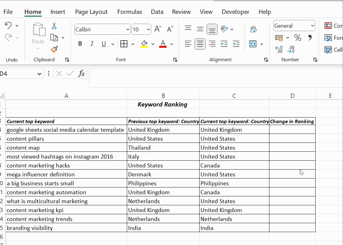
1. In cell D4, input the formula =B4=C4 and press Enter.
2. Drag the formula down to the end of the table.

This formula returns TRUE for matching values and FALSE for differing values.

4. Comparing Two Columns with the IF Condition

The IF condition in Excel can also compare two columns. The formula =IF(B4=C4,”Yes”,” ”) returns Yes for matching values and leaves the remaining rows empty.

4.1. Using the IF Condition

This method is useful for clearly marking matches or mismatches.

Formula: =IF(B4=C4,"Yes"," ")

• “Yes”: Indicates a match.
• ” “: Leaves the cell empty if there is no match.

4.2. Identifying Mismatching Values

You can identify mismatching values by including an additional argument:

Formula: =IF(B4=C4,”Yes”,”No”)

• “Yes”: Indicates a match.
• “No”: Indicates a mismatch.

4.3. Comparing for Differences

To compare two columns for differences, replace the equals sign with the non-equality sign (<>):

Formula: =IF(A2<>B2,”Match”,”Not a Match”)

• “Match”: Indicates the values are different.
• “Not a Match”: Indicates the values are the same.

5. Using the EXACT() Function for Case-Sensitive Comparisons

The EXACT() function ensures that comparisons are case-sensitive. In the IF condition example, the formula returned Yes for matching results with different capitalizations.

5.1. Implementing EXACT() with IF()

To ensure identical capitalizations, use the EXACT() function when comparing two Excel columns with IF().

Formula: =IF(EXACT(B4,C4), “Match”, “Mismatched”)

• “Match”: Indicates a case-sensitive match.
• “Mismatched”: Indicates a mismatch in capitalization or value.

5.2. Understanding the EXACT() Function

The EXACT() function compares two text strings and returns TRUE only if they are identical, including capitalization.

Syntax: =EXACT(text1,text2)

Both arguments, text1 and text2, are required.

6. Compare Two Columns in Excel Using Conditional Formatting

Conditional formatting can highlight data present in both columns without needing a third column to display results.

6.1. Applying Conditional Formatting

To use conditional formatting, follow these steps:

1. Click Home, then Styles.
2. Select Conditional Formatting → Highlight Cell Rules → Duplicate Values.
3. Choose the desired formatting condition from the drop-down menu.

6.2. Options

Apply the formatting condition to the selected cells. Choose either Duplicate or Unique.

• Duplicate: Highlights values present in both columns.
• Unique: Highlights unique values.

6.3. Custom Formatting

Choose Custom Format to highlight cells with a color of your choice.

6.4. Clearing Formatting

To clear the formatting, click Conditional Formatting → Clear Rules → Clear Rules from Selected Cells.

6.5. Highlighting Duplicate Values

To highlight names present in both columns, choose Duplicate and select a highlighting option (e.g., filling with color, changing text color, or changing the cell border).

6.6. Highlighting Unique Values

If you are interested in highlighting cells with data that is not repeated, choose Unique from the drop-down list and apply a highlighting option.

7. Using the LOOKUP Function to Compare Two Columns

The LOOKUP function searches for a specific value in a row or column and returns the corresponding value from another row or column. Various lookup functions include HLOOKUP, VLOOKUP, and XLOOKUP. The XLOOKUP function combines both LOOKUP and VLOOKUP.

7.1. Applying VLOOKUP()

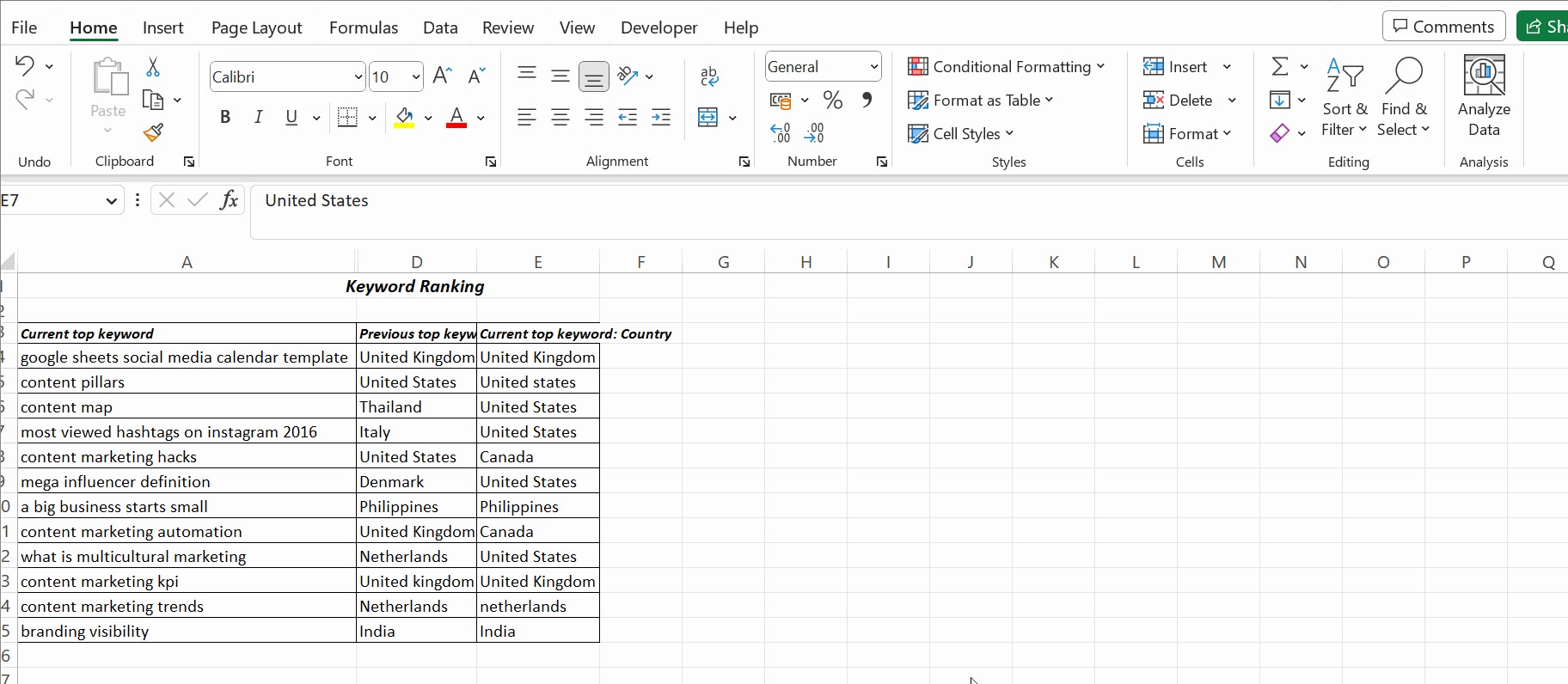
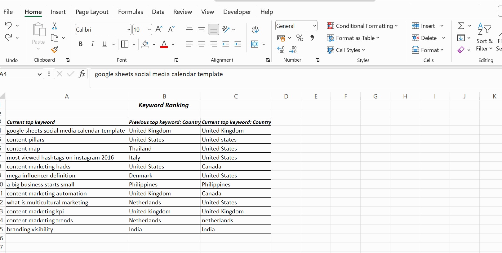
The example below compares two columns in Excel for differences using VLOOKUP(). Column A contains a list of top keywords in a blog, and column B is the parent keyword.

The VLOOKUP() is applied in cell C4 as =VLOOKUP(A4, £B£4:£B£15,1,0). Drag the cell to apply the formula to all cells below C4. You will find the result in column C with the current and matching parent keywords.

7.2. Understanding the Formula

The formula to compare two columns using VLOOKUP is as follows:

VLOOKUP(A4,..,..,..): This takes the value in cell A4.

VLOOKUP(A4, £B£4:£B£15,..,..): This compares all values in cells from B4 to B15. The cells in range B4:B15 are locked using absolute references.

VLOOKUP(A4, £B£4:£B£15,1,..): The third argument is the col_index_num, which mentions the position of the column to compare from the lookup value A4.

VLOOKUP(A4, £B£4:£B£15,1,0): The last argument takes a logical value, either 0 or 1. If you wish to find the exact match, mention 0. If you want VLOOKUP() to return a closest match sorted in ascending order, mention 1 in this argument.

8. VLOOKUP for Identifying Matching Data

VLOOKUP is invaluable for comparing data across two columns by identifying matching entries.

8.1. Formula and Syntax

The VLOOKUP function searches for a value in one column and returns a corresponding value from another column. This is particularly useful when you need to determine if a value from one column exists in another. The syntax is as follows:

=VLOOKUP(lookup_value, table_array, col_index_num, [range_lookup])

• lookup_value: The value you want to search for.
• table_array: The range of cells where you want to search.
• col_index_num: The column number in the range from which to return a value.
• range_lookup: A logical value that specifies whether you want an exact or approximate match (FALSE for exact match).

8.2. Example Scenario

Suppose you have two columns: Column A contains a list of product IDs, and Column B contains a list of customer IDs. You want to find the customer ID associated with a specific product ID.

=VLOOKUP(A2, B:C, 2, FALSE)

In this example:

• A2 is the product ID you are looking up.
• B:C is the range containing the customer IDs.
• 2 indicates that you want to retrieve the customer ID from the second column of the range.
• FALSE specifies that you want an exact match.

If the product ID in A2 is found in Column B, the formula returns the corresponding customer ID from Column C. If not found, it returns an error.

8.3. Handling Errors

When the lookup_value is not found in the table_array, VLOOKUP returns a #N/A error. To handle this, you can use the IFERROR function.

=IFERROR(VLOOKUP(A2, B:C, 2, FALSE), "Not Found")

This formula will return “Not Found” instead of #N/A if the product ID is not found.

9. MATCH Function for Finding the Position of a Value

The MATCH function finds the position of a specified value within a range of cells. This is useful for determining if a value from one column exists in another and identifying its location.

9.1. Formula and Syntax

The syntax for the MATCH function is:

=MATCH(lookup_value, lookup_array, [match_type])

• lookup_value: The value you want to find.

• lookup_array: The range of cells to search within.

• match_type: Specifies how Excel should match the lookup_value:

  • 0: Exact match (most common).
  • 1: Finds the largest value less than or equal to the lookup_value (requires the array to be sorted in ascending order).
  • -1: Finds the smallest value greater than or equal to the lookup_value (requires the array to be sorted in descending order).

9.2. Example Scenario

Suppose you have two columns: Column A contains a list of names, and Column B contains another list of names. You want to find if a name from Column A exists in Column B and, if so, its position.

=MATCH(A2, B:B, 0)

In this example:

• A2 is the name you are looking up.
• B:B is the range of cells (Column B) where you are searching for the name.
• 0 specifies that you want an exact match.

If the name in A2 is found in Column B, the formula returns the position of the name in Column B. If not found, it returns an error.

9.3. Using MATCH with ISNUMBER

To check if a value from Column A exists in Column B without returning an error, you can combine the MATCH function with the ISNUMBER function.

=ISNUMBER(MATCH(A2, B:B, 0))

This formula returns:

• TRUE: If the name in A2 is found in Column B.
• FALSE: If the name in A2 is not found in Column B.

9.4. Practical Applications

• Validating Data: Checking if values in one list exist in another list to ensure data consistency.
• Finding Positions: Identifying the location of a specific item in a dataset.
• Creating Dynamic Reports: Using the position of a value to retrieve corresponding data from other columns.

10. INDEX and MATCH for Flexible Lookups

Combining the INDEX and MATCH functions provides a flexible and powerful way to perform lookups. Unlike VLOOKUP, INDEX and MATCH can look up values to the left and right, making it more versatile.

10.1. Understanding INDEX and MATCH

• INDEX: Returns the value of a cell in a table based on the row and column number. The syntax is:

  =INDEX(array, row_num, [column_num])

• MATCH: Finds the position of a specified value within a range of cells. The syntax is:

  =MATCH(lookup_value, lookup_array, [match_type])

10.2. Combining INDEX and MATCH

By combining these functions, you can perform lookups based on row and column positions determined dynamically.

Basic Formula:

=INDEX(return_array, MATCH(lookup_value, lookup_array, 0))

• return_array: The range of cells from which to return a value.
• lookup_value: The value to search for.
• lookup_array: The range of cells to search within.
• 0: Specifies an exact match.

10.3. Example Scenario

Suppose you have two columns: Column A contains a list of product names, and Column B contains the corresponding prices. You want to find the price of a specific product.

=INDEX(B:B, MATCH(A2, A:A, 0))

In this example:

• B:B is the range containing the prices (the return array).
• A2 is the product name you are looking up.
• A:A is the range of cells (Column A) where you are searching for the product name.
• 0 specifies that you want an exact match.

This formula finds the position of the product name in Column A and then returns the corresponding price from Column B.

10.4. Advantages of INDEX and MATCH

• Flexibility: Can look up values to the left and right, unlike VLOOKUP, which can only look to the right.
• Efficiency: More efficient than VLOOKUP, especially for large datasets, as it only looks at the necessary columns.
• Robustness: Less prone to errors when columns are inserted or deleted, as it is based on the content rather than the column number.

10.5. Practical Applications

• Dynamic Lookups: Performing lookups in large datasets where column positions may change.
• Two-Way Lookups: Looking up values based on both row and column criteria.
• Complex Data Retrieval: Retrieving data from various tables based on multiple conditions.

11. Comparing Multiple Columns Using Array Formulas

Excel’s array formulas can be used to compare multiple columns simultaneously. Array formulas allow you to perform complex calculations across multiple cells.

11.1. Understanding Array Formulas

Array formulas are entered by pressing Ctrl + Shift + Enter instead of just Enter. This tells Excel to perform the calculation on each element of the array.

11.2. Comparing Multiple Columns for Equality

To check if all values in multiple columns are equal in each row, you can use an array formula with the AND function.

Example Scenario:

Suppose you have three columns: Column A, Column B, and Column C. You want to check if the values in each row are the same across all three columns.

Formula:

=AND(A2:A10=B2:B10, B2:B10=C2:C10)

After entering the formula, press Ctrl + Shift + Enter.

This formula compares the values in columns A and B, and then the values in columns B and C. If all comparisons are TRUE, the formula returns TRUE; otherwise, it returns FALSE.

11.3. Highlighting Differences Using Conditional Formatting

You can use array formulas with conditional formatting to highlight rows where the values in multiple columns are different.

Steps:

1. Select the range of cells you want to format (e.g., A2:C10).

2. Go to Home > Conditional Formatting > New Rule.

3. Select Use a formula to determine which cells to format.

4. Enter the following formula:

   =NOT(AND($A2=$B2, $B2=$C2))

5. Click Format to choose the formatting style (e.g., fill color).

6. Click OK to apply the conditional formatting.

This conditional formatting rule highlights rows where the values in columns A, B, and C are not all equal.

11.4. Counting Matching Rows

To count the number of rows where the values in multiple columns are the same, you can use an array formula with the SUM and IF functions.

Formula:

=SUM(IF((A2:A10=B2:B10)*(B2:B10=C2:C10), 1, 0))

After entering the formula, press Ctrl + Shift + Enter.

This formula checks each row to see if the values in columns A, B, and C are equal. If they are, it assigns a value of 1; otherwise, it assigns a value of 0. The SUM function then adds up all the 1s to give you the total number of matching rows.

11.5. Practical Applications

• Data Validation: Ensuring consistency across multiple columns of data.
• Identifying Discrepancies: Highlighting rows where data is inconsistent.
• Reporting: Counting the number of matching rows for summary reports.

12. Advanced Filtering for Complex Comparisons

Excel’s advanced filtering feature allows you to perform complex comparisons between columns based on multiple criteria.

12.1. Setting Up Advanced Filtering

To use advanced filtering, you first need to set up a criteria range. The criteria range should include the column headers you want to filter and the conditions you want to apply.

Steps:

1. Copy the headers of the columns you want to compare to a new location in your worksheet.
2. Underneath the headers, enter the criteria for your comparison.

Example Scenario:

Suppose you have three columns: Column A (Product ID), Column B (Sales), and Column C (Budget). You want to filter the data to show only the rows where the sales are greater than the budget.

Criteria Range:

Product ID	Sales	Budget
	>B2	>C2

12.2. Applying Advanced Filtering

1. Select the data range you want to filter (e.g., A1:C10).
2. Go to Data > Advanced.
3. In the Advanced Filter dialog box:
   • Choose Filter the list, in-place or Copy to another location.
   • Set the List range to your data range (e.g., A1:C10).
   • Set the Criteria range to your criteria range (e.g., E1:G2).
   • If you chose Copy to another location, set the Copy to range.
4. Click OK to apply the filter.

12.3. Complex Criteria

You can use multiple criteria to perform more complex comparisons. For example, you can filter the data to show rows where the sales are greater than the budget and the product ID starts with “P”.

Criteria Range:

Product ID	Sales	Budget
P*	>B2	>C2

In this criteria range, “P*” in the Product ID column means that the filter will only show rows where the Product ID starts with “P”.

12.4. Using Formulas in Criteria

You can also use formulas in the criteria range to perform more advanced comparisons. For example, you can filter the data to show rows where the sales are more than 10% greater than the budget.

Criteria Range:

Product ID	Sales	Budget
	>(1.1*C2)

In this criteria range, >(1.1*C2) in the Sales column means that the filter will only show rows where the sales are more than 110% of the budget.

12.5. Practical Applications

• Data Analysis: Performing complex comparisons between columns to identify trends and patterns.
• Reporting: Filtering data based on multiple criteria to generate specific reports.
• Data Validation: Identifying rows where data does not meet certain criteria.

13. Power Query for Data Transformation and Comparison

Power Query is a powerful data transformation and analysis tool in Excel. It can be used to compare columns, clean data, and perform complex transformations.

13.1. Importing Data into Power Query

To use Power Query, you first need to import your data into the Power Query Editor.

Steps:

1. Select the data range you want to import.
2. Go to Data > From Table/Range.
3. In the Create Table dialog box, make sure the My table has headers box is checked, and click OK.

This opens the Power Query Editor.

13.2. Comparing Columns in Power Query

You can add a custom column to compare two columns and return a value based on the comparison.

Steps:

1. In the Power Query Editor, go to Add Column > Custom Column.

2. In the Custom Column dialog box:

   • Enter a name for the new column (e.g., “Comparison”).
   • Enter the following formula:

   if [ColumnA] = [ColumnB] then "Match" else "Mismatch"

3. Click OK to add the custom column.

This adds a new column that shows “Match” if the values in ColumnA and ColumnB are equal, and “Mismatch” if they are not.

13.3. Conditional Columns

You can also use conditional columns to perform more complex comparisons.

Steps:

1. In the Power Query Editor, go to Add Column > Conditional Column.
2. In the Add Conditional Column dialog box:
   • Set the conditions for your comparison. For example:
     • If Column Name equals ColumnA, Operator equals, Value equals [ColumnB], then Output “Match”.
     • Otherwise, Output “Mismatch”.
3. Click OK to add the conditional column.

13.4. Merging Queries

You can merge two queries to compare data from different tables.

Steps:

1. Go to Home > Merge Queries.
2. In the Merge dialog box:
   • Select the primary table and the column to merge on.
   • Select the secondary table and the corresponding column to merge on.
   • Choose the join kind (e.g., Left Outer, Right Outer, Inner).
3. Click OK to merge the queries.

This merges the two tables based on the selected columns, allowing you to compare data from both tables.

13.5. Practical Applications

• Data Cleaning: Removing inconsistencies and errors from data.
• Data Transformation: Converting data into a format suitable for analysis.
• Data Integration: Combining data from multiple sources into a single table.

14. Comparing Data with Third-Party Add-ins

Several third-party add-ins are available for Excel that can simplify the process of comparing data. These add-ins often offer advanced features and user-friendly interfaces.

14.1. Popular Add-ins

• ASAP Utilities: A popular add-in that provides a wide range of tools for data analysis, including column comparison.
• Kutools for Excel: Offers various functions, including tools for comparing and merging data.
• Ablebits Ultimate Suite for Excel: Includes tools for comparing, cleaning, and managing data.

14.2. Features of Add-ins

These add-ins often provide features such as:

• Side-by-side comparison: Displaying two columns or tables side by side for easy comparison.
• Highlighting differences: Automatically highlighting differences between data.
• Merging data: Combining data from multiple sources into a single table.
• Data cleaning: Removing inconsistencies and errors from data.

14.3. Using Add-ins

To use an add-in, you first need to install it in Excel. Once installed, the add-in will appear in the Excel ribbon, and you can access its features from there.

14.4. Practical Applications

• Data Analysis: Simplifying complex data analysis tasks.
• Reporting: Generating reports with advanced formatting and customization options.
• Data Management: Managing and organizing large datasets more efficiently.

15. Practical Examples and Scenarios

To illustrate the use of different comparison methods, consider the following scenarios:

1. Inventory Management: Compare two lists of product codes to identify missing or duplicate items. Use conditional formatting or VLOOKUP to highlight differences.
2. Sales Data Analysis: Compare sales figures for two different periods to identify trends. Use array formulas to calculate percentage changes and highlight significant variations.
3. Customer Data Validation: Compare customer data from two different sources to ensure consistency. Use Power Query to merge and clean the data.
4. Budget vs. Actual Comparison: Compare budgeted amounts with actual expenses to identify variances. Use advanced filtering to show rows where actual expenses exceed the budget by a certain percentage.

16. Best Practices for Comparing Columns in Excel

To ensure accurate and efficient comparisons, follow these best practices:

1. Prepare Your Data: Clean and format your data before comparing it. Remove any inconsistencies or errors.
2. Choose the Right Method: Select the comparison method that is most appropriate for your data and analysis goals.
3. Use Clear Formulas: Use clear and well-documented formulas.
4. Test Your Formulas: Test your formulas on a small sample of data before applying them to the entire dataset.
5. Use Conditional Formatting: Use conditional formatting to highlight differences and make your analysis more visual.
6. Document Your Steps: Document your steps so that you can easily reproduce your analysis in the future.

17. Automating Comparisons with VBA Macros

VBA (Visual Basic for Applications) macros can automate repetitive tasks in Excel, including column comparisons.

17.1. Understanding VBA

VBA is a programming language that allows you to write code to automate tasks in Excel.

17.2. Writing a VBA Macro for Column Comparison

Here’s an example of a VBA macro that compares two columns and highlights differences:

Sub CompareColumns()
    Dim ws As Worksheet
    Dim lastRow As Long
    Dim i As Long

    ' Set the worksheet
    Set ws = ThisWorkbook.Sheets("Sheet1")

    ' Get the last row in column A
    lastRow = ws.Cells(Rows.Count, "A").End(xlUp).Row

    ' Loop through the rows
    For i = 2 To lastRow ' Assuming headers are in row 1
        ' Compare columns A and B
        If ws.Cells(i, "A").Value <> ws.Cells(i, "B").Value Then
            ' Highlight the row
            ws.Rows(i).Interior.Color = RGB(255, 0, 0) ' Red
        End If
    Next i
End Sub

17.3. How to Use the Macro

1. Open the VBA Editor (Press Alt + F11).
2. Insert a new module (Insert > Module).
3. Paste the code into the module.
4. Modify the code as needed for your specific requirements (e.g., change the worksheet name, column letters, or highlighting color).
5. Run the macro by pressing F5 or clicking the Run button.

17.4. Practical Applications

• Automating Repetitive Tasks: Automating tasks that you perform frequently.
• Customizing Excel: Adding custom functions and features to Excel.
• Creating Dynamic Reports: Creating dynamic reports that update automatically.

18. Common Mistakes to Avoid

When comparing columns in Excel, it’s important to avoid common mistakes that can lead to inaccurate results.

18.1. Ignoring Data Types

Make sure that the data types in the columns you are comparing are the same. For example, if one column contains numbers and the other column contains text, you may need to convert the data types before comparing them.

18.2. Not Cleaning Data

Clean your data before comparing it. Remove any inconsistencies or errors, such as extra spaces, inconsistent capitalization, or incorrect formatting.

18.3. Using Incorrect Formulas

Use the correct formulas for your comparison. Make sure that you understand how the formulas work and that they are appropriate for your data and analysis goals.

18.4. Not Testing Formulas

Test your formulas on a small sample of data before applying them to the entire dataset. This will help you identify any errors and ensure that your formulas are working correctly.

18.5. Overlooking Case Sensitivity

Be aware of case sensitivity when comparing text data. Use the EXACT function if you need to perform a case-sensitive comparison.

18.6. Forgetting to Use Absolute References

Use absolute references when necessary to prevent formulas from changing when you copy them to other cells.

18.7. Not Documenting Steps

Document your steps so that you can easily reproduce your analysis in the future.

19. FAQ

19.1. How do I compare two columns in Excel for differences?

You can compare two columns in Excel for differences using the IF condition. The formula =IF(A2<>B2, "Different", "Same") returns “Different” if the values in columns A and B are different, and “Same” if they are the same.

19.2. How can I highlight differences between two columns in Excel?

You can highlight differences between two columns in Excel using conditional formatting. Select the range of cells you want to format, go to Home > Conditional Formatting > New Rule, and use a formula to determine which cells to format.

19.3. How do I compare two columns in Excel and return a third value?

You can compare two columns in Excel and return a third value using the INDEX and MATCH functions. Use the MATCH function to find the position of a value in one column, and then use the INDEX function to return the corresponding value from another column.

19.4. Can I compare two columns in Excel for case-sensitive matches?

Yes, you can compare two columns in Excel for case-sensitive matches using the EXACT function. The formula =EXACT(A2, B2) returns TRUE if the values in columns A and B are exactly the same, including case, and FALSE if they are not.

19.5. How do I compare two columns in Excel and ignore blank cells?

You can compare two columns in Excel and ignore blank cells using the IF and ISBLANK functions. The formula =IF(OR(ISBLANK(A2), ISBLANK(B2)), "", IF(A2=B2, "Match", "Mismatch")) returns “” if either cell is blank, “Match” if the values are the same, and “Mismatch” if they are different.

19.6. How to compare three or more columns in Excel?

To find matches in all cells when the table has three or more columns, use an IF() with AND statement. The formula is =IF(AND(A2=B2, A2=C2), “Full match”, “”).

The formula to find matches in any two cells in the same row is =IF(OR(A2=B2, B2=C2, A2=C2), “Match”, “”).

20. Conclusion

Comparing two columns in Excel is a task that can be accomplished in many ways. From simple formulas to advanced features, Excel provides the tools necessary to perform accurate and efficient comparisons. By understanding the different methods and following best practices, you can streamline your data analysis and make informed decisions. If you are looking for a solution to compare different choices, visit COMPARE.EDU.VN today to find detailed and objective comparisons that will help you make the right decision. We are located at 333 Comparison Plaza, Choice City, CA 90210, United States. Contact us via Whatsapp: +1 (626) 555-9090 or visit our website: compare.edu.vn

So, whether you’re validating data, identifying discrepancies, or generating reports, mastering column comparison techniques in Excel can significantly enhance your productivity and accuracy.