How Do I Excel Compare Two Columns For Differences?

Excel Compare Two Columns For Differences by using formulas like IF and COUNTIF, conditional formatting, or specialized tools. Explore comprehensive solutions at COMPARE.EDU.VN for identifying matches and unique entries. Enhance your data analysis with Excel techniques for precise comparisons.

1. Understanding the Need to Compare Columns in Excel

Comparing columns in Excel is a frequent task in data analysis. Whether you’re managing lists of customers, products, or any other type of data, identifying differences is essential. At COMPARE.EDU.VN, we understand the importance of efficiently comparing data. Excel provides various methods, including formulas and conditional formatting. But what if you have two different columns that need to be compared? What are the exact differences?

2. Why Compare Two Columns for Differences?

Comparing two columns for differences helps in several scenarios:

• Data Validation: Ensuring data accuracy by identifying discrepancies between two sources.
• Change Tracking: Monitoring changes in data over time.
• Duplicate Identification: Finding unique entries in different data sets.
• Merge and Sync: Preparing data for merging and synchronization.

Comparing two columns in Excel isn’t just about finding differences; it’s about ensuring the integrity and reliability of your data. COMPARE.EDU.VN offers detailed comparisons to assist users in making decisions with confidence.

3. Intent To Search For The User

Here are five primary search intentions behind the keyword “excel compare two columns for differences”:

1. Method Discovery: Users looking for different methods or techniques in Excel to compare two columns and identify differences.
2. Specific Formula Assistance: Seekers needing precise formulas to find matches and differences between two columns.
3. Conditional Formatting Solutions: Individuals wanting to highlight differences between two columns using Excel’s conditional formatting feature.
4. Step-by-Step Instructions: Users requiring a detailed, step-by-step guide on how to compare two columns for differences effectively.
5. Tool Alternatives: Searchers exploring alternative tools or add-ins that simplify the process of comparing columns in Excel.

4. Method 1: Using the IF Function to Compare Two Columns Row by Row

One of the most straightforward methods to excel compare two columns for differences is by using the IF function. This method is particularly useful when you need to compare corresponding rows in two columns.

4.1. The Basic IF Formula

The IF formula checks if a condition is met and returns one value if true and another value if false. Here’s the basic syntax:

=IF(condition, value_if_true, value_if_false)

4.2. Comparing Columns for Matches

To find matches, the condition checks if the values in two cells are equal. For example, to compare cells A2 and B2, the formula is:

=IF(A2=B2, "Match", "")

This formula will return “Match” if the values in A2 and B2 are the same and a blank cell if they are different.

4.3. Comparing Columns for Differences

To find differences, the condition checks if the values in two cells are not equal. The formula is:

=IF(A2<>B2, "No Match", "")

This formula will return “No Match” if the values in A2 and B2 are different and a blank cell if they are the same.

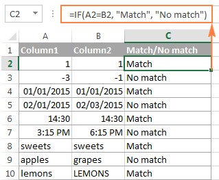
4.4. Combining Matches and Differences

You can combine both matches and differences in one formula:

=IF(A2=B2, "Match", "No Match")

Or

=IF(A2<>B2, "No Match", "Match")

4.5. Applying the Formula to the Entire Column

To apply the formula to all rows, enter the formula in the first row (e.g., C2) and drag the fill handle (the small square at the bottom-right corner of the cell) down to the last row.

4.6. Advantages of the IF Function

• Simple and easy to understand.
• Handles numbers, dates, times, and text strings effectively.

4.7. Limitations of the IF Function

• Ignores case sensitivity.
• Requires manual dragging of the fill handle for large data sets.

5. Method 2: Using the EXACT Function for Case-Sensitive Comparisons

The EXACT function is used to compare two text strings, taking into account case sensitivity.

5.1. The EXACT Formula

The EXACT formula checks if two text strings are identical, including case. Here’s the syntax:

=EXACT(text1, text2)

5.2. Finding Case-Sensitive Matches

To find case-sensitive matches between two columns, the formula is:

=IF(EXACT(A2, B2), "Match", "")

5.3. Finding Case-Sensitive Differences

To find case-sensitive differences, the formula is:

=IF(EXACT(A2, B2), "Match", "Unique")

5.4. Benefits of the EXACT Function

• Provides case-sensitive comparisons.
• Useful for text-based data where case matters.

5.5. Drawbacks of the EXACT Function

• Only works with text strings.
• Can be slower for large data sets compared to the IF function.

6. Method 3: Comparing Multiple Columns for Matches

When you have more than two columns to compare, you can use the AND, OR, and COUNTIF functions.

6.1. Finding Matches in All Cells Within the Same Row Using AND

To find rows where all cells have the same value, use the AND function:

=IF(AND(A2=B2, A2=C2), "Full Match", "")

6.2. Finding Matches in All Cells Within the Same Row Using COUNTIF

A more elegant solution for multiple columns is the COUNTIF function:

=IF(COUNTIF($A2:$E2, $A2)=5, "Full Match", "")

Where 5 is the number of columns you are comparing.

6.3. Finding Matches in Any Two Cells in the Same Row Using OR

To find matches in any two or more cells, use the OR function:

=IF(OR(A2=B2, B2=C2, A2=C2), "Match", "")

6.4. Using COUNTIF for Any Two or More Matches

For many columns, using multiple COUNTIF functions is better:

=IF(COUNTIF(B2:D2,A2)+COUNTIF(C2:D2,B2)+(C2=D2)=0,"Unique","Match")

6.5. Advantages of AND, OR, and COUNTIF

• Flexible for various comparison scenarios.
• COUNTIF is efficient for a large number of columns.

6.6. Limitations of AND, OR, and COUNTIF

• Formulas can become complex for many columns.
• Requires careful construction to ensure accuracy.

7. Method 4: Comparing Two Columns for Matches and Differences Using COUNTIF

To find values in one column but not in another, use the COUNTIF function.

7.1. Basic COUNTIF Formula for Differences

To check if a value in column A exists in column B, use:

=IF(COUNTIF($B:$B, $A2)=0, "No match in B", "")

This formula checks if the value in A2 is found in column B. If COUNTIF returns 0, it means no match is found, and the formula returns “No match in B”.

7.2. Using ISERROR and MATCH for Differences

An alternative approach is using the ISERROR and MATCH functions:

=IF(ISERROR(MATCH($A2,$B$2:$B$10,0)),"No match in B","")

7.3. Using Array Formulas

Another method is using an array formula:

=IF(SUM(--($B$2:$B$10=$A2))=0, " No match in B", "")

Remember to press Ctrl + Shift + Enter to enter it correctly.

7.4. Identifying Matches and Differences in One Formula

To identify both matches and differences, use:

=IF(COUNTIF($B:$B, $A2)=0, "No match in B", "Match in B")

7.5. Benefits of COUNTIF, ISERROR, and MATCH

• Efficient for identifying unique values.
• COUNTIF is easy to understand and implement.

7.6. Drawbacks of COUNTIF, ISERROR, and MATCH

• Can be slow for very large data sets.
• Array formulas require special handling.

8. Method 5: Comparing Two Lists and Pulling Matches Using VLOOKUP, INDEX MATCH, and XLOOKUP

To not only match two columns but also retrieve corresponding data, use the VLOOKUP, INDEX MATCH, or XLOOKUP functions.

8.1. Using VLOOKUP

The VLOOKUP function searches for a value in the first column of a range and returns a value from a specified column in the same row. Here’s the syntax:

=VLOOKUP(lookup_value, table_array, col_index_num, [range_lookup])

Example:

=VLOOKUP(D2, $A$2:$B$6, 2, FALSE)

8.2. Using INDEX MATCH

The INDEX MATCH combination is more flexible than VLOOKUP. INDEX returns a value from a range, and MATCH finds the position of a value in a range.

=INDEX(array, MATCH(lookup_value, lookup_array, [match_type]))

Example:

=INDEX($B$2:$B$6, MATCH($D2, $A$2:$A$6, 0))

8.3. Using XLOOKUP (Excel 2021 and Excel 365)

XLOOKUP is an improved version of VLOOKUP and INDEX MATCH, available in Excel 2021 and Excel 365.

=XLOOKUP(lookup_value, lookup_array, return_array, [if_not_found], [match_mode], [search_mode])

Example:

=XLOOKUP(D2, $A$2:$A$6, $B$2:$B$6)

8.4. Advantages of VLOOKUP, INDEX MATCH, and XLOOKUP

• Efficient for retrieving related data.
• XLOOKUP is more versatile and easier to use.

8.5. Limitations of VLOOKUP, INDEX MATCH, and XLOOKUP

• VLOOKUP has limitations with column positioning.
• INDEX MATCH can be complex for beginners.

9. Method 6: Comparing Two Lists and Highlighting Matches and Differences Using Conditional Formatting

Conditional formatting allows you to highlight cells based on certain criteria.

9.1. Highlighting Matches and Differences in Each Row

To highlight cells in column A that have identical entries in column B in the same row:

1. Select the cells you want to highlight.
2. Go to Conditional Formatting > New Rule… > Use a formula to determine which cells to format.
3. Enter the formula =$B2=$A2.

To highlight differences, use the formula =$B2<>$A2.

9.2. Highlighting Unique Entries in Each List

To highlight items that are only in one list:

1. Select List 1 (column A).
2. Go to Conditional Formatting > New Rule… > Use a formula to determine which cells to format.
3. Enter the formula =COUNTIF($C$2:$C$5, $A2)=0.

Repeat for List 2 (column C) with the formula =COUNTIF($A$2:$A$6, $C2)=0.

9.3. Highlighting Matches (Duplicates) Between Two Columns

To highlight matches:

1. Select List 1 (column A).
2. Go to Conditional Formatting > New Rule… > Use a formula to determine which cells to format.
3. Enter the formula =COUNTIF($C$2:$C$5, $A2)>0.

Repeat for List 2 (column C) with the formula =COUNTIF($A$2:$A$6, $C2)>0.

9.4. Benefits of Conditional Formatting

• Visually highlights matches and differences.
• Easy to set up and customize.

9.5. Drawbacks of Conditional Formatting

• Can slow down Excel with complex rules and large data sets.
• Only provides visual cues, not actual data manipulation.

10. Method 7: Highlighting Row Differences and Matches in Multiple Columns

When comparing values in several columns row-by-row, conditional formatting and the Go To Special feature can be used.

10.1. Highlighting Rows That Have Identical Values in All Columns

Use conditional formatting with one of the following formulas:

=AND($A2=$B2, $A2=$C2)

or

=COUNTIF($A2:$C2, $A2)=3

Where A2, B2, and C2 are the top-most cells and 3 is the number of columns to compare.

10.2. Highlighting Cells with Different Values in Each Individual Row Using Go To Special

1. Select the range of cells you want to compare.
2. On the Home tab, go to Editing group, and click Find & Select > Go To Special…
3. Select Row differences and click the OK button.
4. The cells whose values are different from the comparison cell in each row are colored.

10.3. Advantages of Go To Special and Conditional Formatting

• Quickly highlights differences in multiple columns.
• Easy to use for visual comparisons.

10.4. Limitations of Go To Special and Conditional Formatting

• Go To Special is manual and doesn’t update automatically.
• Conditional formatting can slow down Excel.

11. Method 8: Formula-Free Way to Compare Two Columns/Lists in Excel Using Ablebits

For a formula-free way to compare columns, consider using the Compare Two Tables tool included in Ultimate Suite.

11.1. Steps to Compare Two Lists Using Ablebits

1. Click the Compare Tables button on the Ablebits Data tab.
2. Select the first column/list and click Next.
3. Select the second column/list and click Next.
4. Choose what kind of data to look for:
   • Duplicate values (matches)
   • Unique values (differences)
5. Select the columns for comparison.
6. Choose how to deal with the found items and click Finish. Options include:
   • Highlight with color
   • Identify in the Status column
     

11.2. Benefits of Using Ablebits

• No formulas required.
• Easy to use with a user-friendly interface.
• Offers various options for highlighting and identifying differences.

11.3. Drawbacks of Using Ablebits

• Requires installing an add-in.
• May not be suitable for users who prefer using native Excel functions.

12. Additional Tips and Considerations

• Sorting Data: Sorting your data before comparing can help in identifying patterns and differences more easily.
• Using Filters: Excel’s filter feature can be used to isolate unique entries after comparing columns.
• Data Cleaning: Ensure your data is clean and consistent before comparing. Remove any unnecessary spaces or special characters.
• Performance: For large data sets, consider using array formulas and conditional formatting sparingly to avoid slowing down Excel.
• Check for Errors: Review your formulas and conditional formatting rules to ensure they are correct and provide accurate results.

13. Real-World Applications

• Inventory Management: Comparing inventory lists to identify discrepancies.
• Customer Relationship Management (CRM): Identifying duplicate customer entries.
• Financial Auditing: Comparing financial data to detect fraud or errors.
• Human Resources: Comparing employee lists to identify missing or incorrect information.
• Academic Research: Comparing data sets from different sources to validate findings.

14. Choosing the Right Method

Selecting the right method depends on your specific needs:

• Simple Comparisons: Use the IF function for basic comparisons.
• Case-Sensitive Comparisons: Use the EXACT function.
• Multiple Columns: Use AND, OR, and COUNTIF.
• Unique Values: Use COUNTIF, ISERROR, and MATCH.
• Data Retrieval: Use VLOOKUP, INDEX MATCH, or XLOOKUP.
• Visual Highlighting: Use conditional formatting.
• Formula-Free Solution: Use Ablebits.

15. Frequently Asked Questions (FAQ)

Q1: How do I compare two columns in Excel for exact matches?

Use the EXACT function within an IF formula to perform a case-sensitive comparison. For example: =IF(EXACT(A2, B2), "Match", "No Match").

Q2: Can I compare two columns in different Excel sheets?

Yes, you can reference cells from different sheets in your formulas. For example, =IF(Sheet1!A2=Sheet2!A2, "Match", "No Match").

Q3: How do I ignore case when comparing two columns?

Use the standard IF formula for case-insensitive comparisons. For example: =IF(A2=B2, "Match", "No Match").

Q4: What is the fastest way to compare two large columns in Excel?

Using built-in functions like COUNTIF or conditional formatting can be slow for very large datasets. Consider using a tool like Ablebits’ Compare Two Tables for better performance.

Q5: How do I highlight unique values in two columns?

Use conditional formatting with a formula like =COUNTIF($B:$B, $A2)=0 to highlight unique values in column A compared to column B.

Q6: How do I find differences between two columns and list them?

Use the IF and COUNTIF functions to identify differences, then filter the results to list only the differing values.

Q7: Can I compare two columns for partial matches?

Yes, use functions like SEARCH or FIND within an IF formula to find partial matches. For example: =IF(ISNUMBER(SEARCH(A2, B2)), "Partial Match", "No Match").

Q8: How do I compare two columns and return a value from a third column if there’s a match?

Use VLOOKUP, INDEX MATCH, or XLOOKUP to return a value from another column when a match is found.

Q9: What is the best alternative to using formulas for comparing columns?

Add-ins like Ablebits’ Compare Two Tables provide a user-friendly, formula-free way to compare columns with more features.

Q10: How do I troubleshoot errors when comparing columns in Excel?

Check for typos in your formulas, ensure cell references are correct, and verify that the data types in the columns being compared are consistent.

16. Conclusion: Making Informed Decisions with COMPARE.EDU.VN

Comparing two columns for differences in Excel is a fundamental skill for data analysis. COMPARE.EDU.VN provides a comprehensive guide, covering various methods from basic formulas to advanced tools. By understanding these techniques, you can efficiently validate data, track changes, and identify unique entries.

Remember to choose the method that best fits your specific needs. Whether you prefer the simplicity of the IF function or the advanced features of Ablebits, Excel offers a range of options to suit every scenario.

For more detailed comparisons and to make informed decisions, visit COMPARE.EDU.VN. We are dedicated to providing you with the resources you need to excel in your data analysis tasks.

Address: 333 Comparison Plaza, Choice City, CA 90210, United States

WhatsApp: +1 (626) 555-9090

Website: COMPARE.EDU.VN

Take action now! Visit compare.edu.vn to explore more comparisons and make informed decisions today!