Comparing data in Excel is a common task, and mastering how to compare two columns is crucial for data analysis. Whether you need to identify matches, differences, or extract specific information, this guide provides a comprehensive overview of techniques for effectively comparing two columns in Excel. Brought to you by COMPARE.EDU.VN, we ensure you’re equipped with the best methods for data comparison. Learn effective excel comparison methods to streamline your data analysis process.
1. Understanding the Basics of Excel Column Comparison
Before diving into specific methods, it’s essential to understand the fundamental concepts involved in comparing two columns in Excel. This includes understanding cell references, operators, and basic functions that will be used throughout this guide. Effective comparison of columns requires an understanding of excel formulas.
1.1 Why Compare Columns in Excel?
Comparing columns in Excel allows you to identify discrepancies, duplicates, and unique entries. This is crucial for ensuring data accuracy, validating data integrity, and making informed decisions based on your data. Streamline your data analysis workflow.
1.2 Key Elements for Column Comparison
- Cell References: Understanding absolute ($A$1) vs. relative (A1) cell references is essential for creating formulas that can be applied across multiple rows.
- Comparison Operators: Operators like =, <>, >, <, >=, and <= are used to compare values within cells.
- Basic Functions: Functions like IF, COUNTIF, MATCH, and VLOOKUP are commonly used for performing comparisons.
2. Comparing Two Columns Row-by-Row
Comparing two columns on a row-by-row basis is one of the most common tasks in Excel. This involves checking whether the values in corresponding rows of two columns match or differ.
2.1 Using the IF Function for Basic Comparison
The IF function is a powerful tool for comparing values in two columns. It allows you to specify a condition and return different results based on whether the condition is true or false.
2.1.1 Formula for Matches
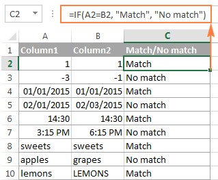
To check for matches in columns A and B, use the following formula in column C:
=IF(A2=B2,"Match","No Match")
This formula compares the values in cells A2 and B2. If they are equal, the formula returns “Match”; otherwise, it returns “No Match”.
2.1.2 Formula for Differences
To check for differences, use the following formula:
=IF(A2<>B2,"Different","Same")
This formula returns “Different” if the values in A2 and B2 are not equal, and “Same” if they are equal.
2.2 Case-Sensitive Comparison with the EXACT Function
The IF function is not case-sensitive. If you need to perform a case-sensitive comparison, use the EXACT function.
2.2.1 Formula for Case-Sensitive Matches
=IF(EXACT(A2,B2),"Match","No Match")
This formula compares the values in A2 and B2 and returns “Match” only if they are exactly the same, including case.
2.2.2 Formula for Case-Sensitive Differences
=IF(EXACT(A2,B2),"Same","Different")
This formula returns “Same” if the values in A2 and B2 are exactly the same, and “Different” otherwise.
2.3 Comparing Multiple Columns Simultaneously
You can extend the comparison to multiple columns using the AND or OR functions in conjunction with the IF function. Excel offers a variety of functions for comparing data in each individual row.
2.3.1 Formula for Matching All Columns
To check if values in columns A, B, and C are the same:
=IF(AND(A2=B2,A2=C2),"Match","No Match")
This formula returns “Match” only if the values in A2, B2, and C2 are all equal.
2.3.2 Formula for Matching Any Two Columns
To check if any two columns match:
=IF(OR(A2=B2,A2=C2,B2=C2),"Match","No Match")
This formula returns “Match” if any of the pairs (A2 and B2, A2 and C2, or B2 and C2) are equal.
3. Comparing Two Columns for Matches and Differences (List Comparison)
When you have two lists of data in separate columns, you might want to identify which values are present in one list but not in the other. This is useful for identifying unique entries or missing data.
3.1 Using COUNTIF to Find Matches
The COUNTIF function is used to count the number of cells within a range that meet a given criteria.
3.1.1 Formula to Find Values in Column A that Exist in Column B
=IF(COUNTIF($B:$B,A2)>0,"Match","No Match")
This formula counts the number of times the value in A2 appears in column B. If the count is greater than 0, it means the value exists in column B, and the formula returns “Match”. Otherwise, it returns “No Match”.
3.1.2 Formula to Find Values in Column A that Do Not Exist in Column B
=IF(COUNTIF($B:$B,A2)=0,"Unique to A","")
This formula counts the number of times the value in A2 appears in column B. If the count is 0, it means the value does not exist in column B, and the formula returns “Unique to A”. Otherwise, it returns an empty string.
3.2 Using MATCH and ISERROR to Find Matches
The MATCH function searches for a specified item in a range of cells and returns the relative position of that item in the range. The ISERROR function checks whether a value is an error and returns TRUE or FALSE.
3.2.1 Formula to Find Values in Column A that Exist in Column B
=IF(ISERROR(MATCH(A2,$B:$B,0)),"No Match","Match")
This formula searches for the value in A2 within column B. If MATCH returns an error (meaning the value is not found), ISERROR returns TRUE, and the formula returns “No Match”. Otherwise, it returns “Match”.
3.2.2 Formula to Find Values in Column A that Do Not Exist in Column B
=IF(ISERROR(MATCH(A2,$B:$B,0)),"Unique to A","")
This formula searches for the value in A2 within column B. If MATCH returns an error (meaning the value is not found), ISERROR returns TRUE, and the formula returns “Unique to A”. Otherwise, it returns an empty string.
4. Pulling Matching Data from One Column to Another
Sometimes, you need to not only compare columns but also retrieve corresponding data from another column based on the match. This can be achieved using VLOOKUP, INDEX MATCH, or XLOOKUP.
4.1 Using VLOOKUP to Retrieve Matching Data
The VLOOKUP function looks for a value in the first column of a range and returns a value from a specified column in the same row.
4.1.1 Formula to Retrieve Data
=VLOOKUP(D2,$A$2:$B$10,2,FALSE)
- D2: The lookup value (the value to search for in column A).
- $A$2:$B$10: The range in which to search (column A) and retrieve data (column B).
- 2: The column number within the range from which to retrieve the data (column B is the second column).
- FALSE: Specifies an exact match.
This formula searches for the value in D2 within column A and returns the corresponding value from column B. If no match is found, it returns an error.
4.2 Using INDEX MATCH to Retrieve Matching Data
The INDEX MATCH combination is a more flexible alternative to VLOOKUP. It uses the MATCH function to find the row number of the matching value and the INDEX function to retrieve the value from that row.
4.2.1 Formula to Retrieve Data
=INDEX($B$2:$B$10,MATCH(D2,$A$2:$A$10,0))
- $B$2:$B$10: The range from which to retrieve the data (column B).
- MATCH(D2,$A$2:$A$10,0): Finds the row number of the matching value in column A.
- D2: The lookup value.
- $A$2:$A$10: The range to search for the lookup value (column A).
- 0: Specifies an exact match.
This formula searches for the value in D2 within column A and returns the corresponding value from column B.
4.3 Using XLOOKUP to Retrieve Matching Data
XLOOKUP is a newer function available in Excel 365 and later versions. It combines the functionality of VLOOKUP and INDEX MATCH and offers additional features.
4.3.1 Formula to Retrieve Data
=XLOOKUP(D2,$A$2:$A$10,$B$2:$B$10,"Not Found")
- D2: The lookup value (the value to search for in column A).
- $A$2:$A$10: The lookup array (the range to search for the lookup value in column A).
- $B$2:$B$10: The return array (the range from which to retrieve the data in column B).
- “Not Found”: The value to return if no match is found.
This formula searches for the value in D2 within column A and returns the corresponding value from column B. If no match is found, it returns “Not Found”.
5. Highlighting Matches and Differences
Conditional formatting allows you to visually highlight matches and differences between columns, making it easier to identify discrepancies and patterns.
5.1 Highlighting Matches in Two Columns
To highlight cells in column A that match the corresponding cells in column B:
- Select the range of cells in column A.
- Go to Home > Conditional Formatting > New Rule.
- Select Use a formula to determine which cells to format.
- Enter the formula
=$A2=$B2. - Click Format and choose a fill color.
- Click OK twice.
This will highlight all cells in column A that have the same value as the corresponding cells in column B.
5.2 Highlighting Differences in Two Columns
To highlight cells in column A that differ from the corresponding cells in column B:
- Select the range of cells in column A.
- Go to Home > Conditional Formatting > New Rule.
- Select Use a formula to determine which cells to format.
- Enter the formula
=$A2<>$B2. - Click Format and choose a fill color.
- Click OK twice.
This will highlight all cells in column A that have different values from the corresponding cells in column B.
5.3 Highlighting Unique Entries in Two Lists
To highlight values that are unique to one list or the other:
- Select the range of cells in column A (List 1).
- Go to Home > Conditional Formatting > New Rule.
- Select Use a formula to determine which cells to format.
- Enter the formula
=COUNTIF($B:$B,A2)=0. - Click Format and choose a fill color.
- Click OK twice.
- Repeat the same steps for column B (List 2), using the formula
=COUNTIF($A:$A,B2)=0.
This will highlight values in each list that do not appear in the other list.
5.4 Highlighting Matches (Duplicates) Between Two Columns
To highlight values that appear in both lists:
- Select the range of cells in column A (List 1).
- Go to Home > Conditional Formatting > New Rule.
- Select Use a formula to determine which cells to format.
- Enter the formula
=COUNTIF($B:$B,A2)>0. - Click Format and choose a fill color.
- Click OK twice.
- Repeat the same steps for column B (List 2), using the formula
=COUNTIF($A:$A,B2)>0.
This will highlight values in each list that appear in the other list.
6. Comparing Multiple Columns and Highlighting Row Differences
When working with multiple columns, you may need to identify rows where the values differ. Excel’s Go To Special feature provides a quick way to highlight these differences.
6.1 Using Go To Special to Highlight Row Differences
- Select the range of cells you want to compare.
- Press Ctrl + G to open the Go To dialog box.
- Click Special.
- Select Row differences and click OK.
- The cells with different values will be selected.
- Click the Fill Color icon on the ribbon and select a color.
This will highlight cells with different values in each row.
7. Advanced Techniques for Column Comparison
Beyond the basic techniques, there are more advanced methods for comparing columns in Excel.
7.1 Array Formulas for Complex Comparisons
Array formulas allow you to perform complex calculations on ranges of cells. They are entered by pressing Ctrl + Shift + Enter.
7.1.1 Formula to Find Values in Column A That Do Not Exist in Column B (Array Formula)
=IF(SUM(--($B$2:$B$10=A2))=0,"Unique to A","")
This array formula compares the value in A2 with each value in the range B2:B10. If the sum of matches is 0, it means the value does not exist in column B.
7.2 Using Power Query for Data Comparison
Power Query is a powerful data transformation and analysis tool in Excel. It can be used to compare and merge data from multiple sources.
7.2.1 Steps to Compare Columns Using Power Query
- Select the data in column A and go to Data > From Table/Range.
- In the Power Query Editor, rename the query to “ListA”.
- Close and Load To > Only Create Connection.
- Repeat steps 1-3 for column B, naming the query “ListB”.
- Go to Data > Get Data > Combine Queries > Merge.
- Select “ListA” as the first table and “ListB” as the second table.
- Select the column to compare in both tables.
- Choose the join kind (e.g., Left Anti to find values only in ListA).
- Expand the resulting column to see the matching values.
8. Simplifying Column Comparison with COMPARE.EDU.VN
Comparing columns in Excel can be time-consuming and complex. COMPARE.EDU.VN simplifies this process by providing a user-friendly platform for comparing data. Whether you’re comparing product features, pricing, or any other type of data, our platform offers intuitive tools and visualizations to help you make informed decisions. Compare multiple options to help you choose the right one.
8.1 Benefits of Using COMPARE.EDU.VN
- Easy-to-Use Interface: Our platform is designed to be intuitive and easy to navigate, even for users with limited Excel experience.
- Comprehensive Comparisons: We provide detailed comparisons across multiple criteria, ensuring you have all the information you need.
- Visualizations: Our platform includes charts, graphs, and other visualizations to help you quickly identify patterns and trends.
- Objective Data: We provide objective, data-driven comparisons to help you avoid bias and make informed decisions.
8.2 How COMPARE.EDU.VN Works
- Upload Your Data: Simply upload your Excel data to our platform.
- Select Columns to Compare: Choose the columns you want to compare.
- View Results: Our platform generates a comprehensive comparison report with detailed analysis and visualizations.
9. Real-World Applications of Column Comparison
Column comparison is a versatile technique with numerous real-world applications across various industries.
9.1 Data Validation
Ensuring data accuracy and consistency is crucial in many fields. Column comparison can be used to validate data entries, identify errors, and maintain data integrity.
9.1.1 Example: Validating Customer Data
Compare customer data from two different sources to identify discrepancies and ensure that customer information is consistent across systems.
9.2 Identifying Duplicates
Identifying and removing duplicate entries is essential for maintaining data quality and avoiding errors.
9.2.1 Example: Removing Duplicate Product Listings
Compare product listings from different suppliers to identify and remove duplicate entries, ensuring that your product catalog is accurate and up-to-date.
9.3 Comparing Product Features
When evaluating different products or services, it’s important to compare their features and specifications.
9.3.1 Example: Comparing Smartphone Specifications
Compare the specifications of different smartphones (e.g., screen size, camera resolution, battery life) to determine which one best meets your needs.
9.4 Analyzing Financial Data
Column comparison can be used to analyze financial data, identify trends, and detect anomalies.
9.4.1 Example: Comparing Monthly Sales Figures
Compare monthly sales figures over a period of time to identify trends and patterns in sales performance.
10. Common Mistakes to Avoid
While comparing columns in Excel, it’s important to avoid common mistakes that can lead to inaccurate results.
10.1 Not Using Absolute Cell References
When copying formulas, it’s essential to use absolute cell references ($A$1) to prevent the references from changing.
10.2 Ignoring Case Sensitivity
Remember that the IF function is not case-sensitive. Use the EXACT function for case-sensitive comparisons.
10.3 Forgetting to Press Ctrl + Shift + Enter for Array Formulas
Array formulas must be entered by pressing Ctrl + Shift + Enter. Otherwise, they will not work correctly.
10.4 Not Validating Data Types
Ensure that the data types in the columns you are comparing are consistent. Comparing numbers to text can lead to unexpected results.
11. Frequently Asked Questions (FAQs)
1. How do I compare two columns in Excel for matches and differences?
Use the IF and COUNTIF functions to identify matches and differences between two columns. For example, =IF(COUNTIF($B:$B,A2)>0,"Match","No Match") checks if the value in A2 exists in column B.
2. How do I highlight unique entries in two columns?
Use conditional formatting with the COUNTIF function. For example, =COUNTIF($B:$B,A2)=0 highlights values in column A that do not exist in column B.
3. Can I compare two columns in Excel for case-sensitive matches?
Yes, use the EXACT function in conjunction with the IF function. For example, =IF(EXACT(A2,B2),"Match","No Match") performs a case-sensitive comparison between A2 and B2.
4. How can I retrieve data from one column based on a match in another column?
Use VLOOKUP, INDEX MATCH, or XLOOKUP to retrieve data. For example, =VLOOKUP(D2,$A$2:$B$10,2,FALSE) searches for the value in D2 within column A and returns the corresponding value from column B.
5. How do I compare multiple columns simultaneously?
Use the AND or OR functions in conjunction with the IF function. For example, =IF(AND(A2=B2,A2=C2),"Match","No Match") checks if the values in A2, B2, and C2 are all equal.
6. What is the best way to highlight row differences in Excel?
Use Excel’s Go To Special feature to quickly highlight cells with different values in each row.
7. Are there any tools that simplify column comparison in Excel?
Yes, COMPARE.EDU.VN offers a user-friendly platform for comparing data, with intuitive tools and visualizations to help you make informed decisions.
8. What are some common mistakes to avoid when comparing columns in Excel?
Avoid not using absolute cell references, ignoring case sensitivity, forgetting to press Ctrl + Shift + Enter for array formulas, and not validating data types.
9. How can I use Power Query to compare two columns?
Use Power Query to merge and compare data from multiple sources. You can use different join kinds to find values that are unique to one list or the other.
10. What are some real-world applications of column comparison?
Column comparison can be used for data validation, identifying duplicates, comparing product features, and analyzing financial data.
12. Conclusion
Mastering the techniques for comparing two columns in Excel is essential for data analysis and decision-making. Whether you’re identifying matches, differences, or retrieving specific information, the methods outlined in this guide will help you effectively compare your data. Remember to validate data types before comparing.
For a simpler, more intuitive way to compare data, visit COMPARE.EDU.VN. Our platform provides comprehensive comparisons, visualizations, and objective data to help you make informed decisions. Contact us at 333 Comparison Plaza, Choice City, CA 90210, United States or via Whatsapp at +1 (626) 555-9090. Visit our website at COMPARE.EDU.VN to learn more.
Ready to make smarter decisions? Visit compare.edu.vn today and start comparing your options with ease and confidence!