
In the realm of data analysis, especially when using tools like Microsoft Excel, the ability to compare data sets is paramount. Whether you’re auditing data, reconciling lists, or simply identifying discrepancies, knowing how to effectively compare columns is crucial. While manual comparison is tedious and error-prone, Excel offers a range of powerful formulas to automate this process, saving you time and enhancing accuracy. This guide delves into various Excel formulas you can use to compare columns, ensuring you can tackle any data comparison task with confidence.
Understanding Column Comparison in Excel
Comparing columns in Excel essentially involves checking corresponding cells across different columns to identify similarities or differences. This could range from simple equality checks to more complex comparisons based on specific criteria. Formulas are the backbone of efficient column comparison in Excel, allowing you to perform these checks quickly and dynamically.
Why Use Formulas for Comparison?
- Efficiency: Formulas automate the comparison process, handling large datasets in seconds.
- Accuracy: Eliminates manual errors inherent in visual inspection.
- Flexibility: Formulas can be customized to perform various types of comparisons, from exact matches to partial matches.
- Dynamic Results: As data changes, formulas automatically recalculate and update comparison results.
Let’s explore the essential formulas and techniques to compare columns effectively in Excel.
Essential Excel Formulas for Column Comparison
Excel provides a suite of formulas designed to handle different comparison needs. We’ll explore some of the most effective methods:
1. Conditional Formatting with Formulas
Conditional formatting is a visual way to highlight cells based on specific criteria. When combined with formulas, it becomes a powerful tool for visually comparing columns.
Step-by-Step Guide:
-
Select the column(s) you want to format. For example, if you want to compare Column A to Column B and highlight differences in Column A, select Column A.
-
Navigate to Conditional Formatting: Go to the “Home” tab on the Excel ribbon, then click on “Conditional Formatting”.
-
Create a New Rule: Select “New Rule” from the dropdown menu.
-
Use a formula to determine which cells to format: In the “New Formatting Rule” dialog box, choose “Use a formula to determine which cells to format”.
-
Enter your comparison formula: In the formula box, enter a formula to compare the current cell in Column A with the corresponding cell in Column B. For example, to highlight cells in Column A that are different from Column B, use the formula:
=A1<>B1. (Assuming you selected column A starting from A1). -
Set the formatting: Click on the “Format” button to choose how you want the different cells to be highlighted (e.g., fill color, font color, etc.).
-
Click “OK” in both dialog boxes to apply the conditional formatting.
Now, any cell in Column A that does not match its corresponding cell in Column B will be formatted according to your chosen style, visually highlighting the differences.
2. Using the Equals (=) Operator in Formulas
The equals operator is the most basic formula for comparing cells. It returns TRUE if the cells are identical and FALSE otherwise.
Step-by-Step Guide:
-
Insert a new column next to the columns you want to compare. This will be your “Result” column.
-
In the first cell of the Result column (e.g., C1), enter the formula:
=A1=B1(assuming your data starts in row 1 and you are comparing Column A and Column B). -
Drag the fill handle (the small square at the bottom-right of the cell) down to apply the formula to the rest of the rows.
The Result column will now display TRUE for rows where Column A and Column B are the same, and FALSE where they differ.
Enhancing with the IF Formula
You can make the results more descriptive by using the IF formula to display custom messages instead of TRUE and FALSE.
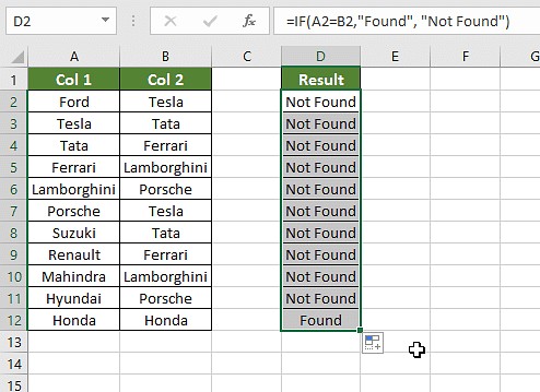
Modified Formula in C1: =IF(A1=B1, "Match", "No Match")
{width=494 height=359}
*Alt Text: Excel sheet displaying the IF formula `=IF(A1=B1, "Match", "No Match")` in cell C1, showing custom text results "Match" and "No Match" based on column comparison.*This formula checks if A1 equals B1. If TRUE, it displays “Match”; if FALSE, it displays “No Match”. This provides clearer, text-based comparison results.
3. Leveraging the VLOOKUP Formula
The VLOOKUP function is primarily used to find values in a table, but it can also be adapted for column comparison, especially when you need to check if values from one column exist in another.
Formula Structure: =VLOOKUP(lookup_value, table_array, col_index_num, [range_lookup])
For column comparison, we’ll use it to check if values in one column are present in another.
Step-by-Step Guide:
-
In the Result column (e.g., C1), enter the formula:
=VLOOKUP(A1, B:B, 1, FALSE)(assuming you are checking if values in Column A exist in Column B).A1: The value to look up (first cell in Column A).B:B: The table array, which is the entire Column B where we are looking for matches.1: The column index number (since we are looking within Column B itself, it’s the first column).FALSE: For an exact match.
-
Drag the fill handle down to apply the formula to all rows.
If a value from Column A is found in Column B, VLOOKUP will return that value. If not found, it returns an error #N/A.
Handling Errors with IFERROR
To replace errors with more user-friendly messages, use the IFERROR function:
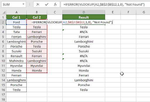
Modified Formula in C1: =IFERROR(VLOOKUP(A1, B:B, 1, FALSE), "Not Found")
{width=512 height=350}
*Alt Text: Excel sheet demonstrating the use of IFERROR with VLOOKUP, formula `=IFERROR(VLOOKUP(A1, B:B, 1, FALSE), "Not Found")` in cell C1, showing "Not Found" instead of #N/A errors.*This formula returns “Not Found” if VLOOKUP results in an error, indicating the value from Column A is not in Column B. Otherwise, it returns the matched value.
Using Wildcards in VLOOKUP for Partial Matches
In scenarios where you need to compare columns with slight variations in text (e.g., “Ford India” vs. “Ford”), you can use wildcards with VLOOKUP.
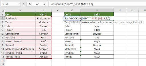
Example Formula: =IFERROR(VLOOKUP(A1&"*", B:B, 1, FALSE), "Not Found")
{width=512 height=234}
*Alt Text: Excel sheet showing VLOOKUP formula with wildcard `*`, `=IFERROR(VLOOKUP(A1&"*", B:B, 1, FALSE), "Not Found")` in cell C1, enabling partial match comparison.*Appending &"*" to A1 allows VLOOKUP to find matches even if Column B contains values that start with the text in A1 but have additional characters.
4. Utilizing the IF Formula for Conditional Outcomes
We’ve already seen how to use IF with the equals operator. The IF formula is highly versatile and can be used for more complex conditional comparisons.
Formula Structure: =IF(logical_test, value_if_true, value_if_false)
Example: Comparing Car Brands
Suppose you want to compare car brands in Column A and Column B and display “Same Brand” if they match, and “Different Brand” if they don’t.
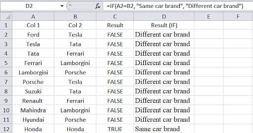
Formula in C1: =IF(A1=B1, "Same Brand", "Different Brand")
{width=512 height=270}
*Alt Text: Excel sheet displaying the IF formula `=IF(A1=B1, "Same Brand", "Different Brand")` in column D, showing text results "Same car brands" or "Different car brands" based on car brand comparison in columns A and B.*This formula checks if the car brand in A1 is the same as in B1. It returns “Same Brand” if TRUE, and “Different Brand” if FALSE.
5. Employing the EXACT Formula for Case-Sensitive Comparison
The EXACT formula is specifically designed for case-sensitive comparisons. It returns TRUE only if two strings are exactly the same, including case, and FALSE otherwise.
Formula Structure: =EXACT(text1, text2)
Example: Case-Sensitive Comparison
To compare values in Column A and Column B case-sensitively:
Formula in C1: =EXACT(A1, B1)
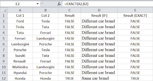{width=512 height=271}
*Alt Text: Excel sheet showing the EXACT formula `=EXACT(A1, B1)` in column C, displaying TRUE or FALSE results based on case-sensitive comparison of columns A and B.*If A1 contains “Honda” and B1 contains “honda”, the EXACT formula will return FALSE because of the case difference. If both are “Honda”, it will return TRUE.
Choosing the Right Formula for Your Scenario
The best formula for column comparison depends on your specific needs. Here’s a guide to help you choose:
Scenario 1: Row-by-Row Comparison for Matches and Differences
For simple row-by-row comparison to find matches or differences, use:
-
=IF(A1=B1, "Match", " ")or=IF(A1=B1, "Match", "No Match")for basic comparison. -
=IF(A1<>B1, "No Match", " ")to specifically highlight differences. -
=IF(EXACT(A1, B1), "Match", " ")for case-sensitive comparison.
Scenario 2: Comparing Multiple Columns in Excel
To compare more than two columns for matches across rows, use:
=IF(AND(A1=B1, A1=C1), "Complete Match", " ")for checking if all columns match.=IF(COUNTIF(A1:E1, A1)=5, "Complete Match", " ")(adjust range and count as needed) for a more scalable approach when comparing many columns.
For finding rows with at least two matching cells among multiple columns:
=IF(OR(A1=B1, B1=C1, A1=C1), "Match", "")=IF(COUNTIF(B1:D1,A1)+COUNTIF(C1:D1,B1)+(C1=D1)=0,"Unique","Match")for identifying unique rows versus rows with matches.
Scenario 3: Comparing Two Columns for Unique Values
To find values in Column A that are not present in Column B:
=IF(COUNTIF(B:B, A1)=0, "Not in Column B", "")=IF(ISERROR(MATCH(A1,B:B,0)),"Not in Column B","")
For a combined result showing both matches and uniques:
=IF(COUNTIF(B:B, A1)=0, "Not in Column B", "Present in Column B")
Scenario 4: Comparing Two Lists and Extracting Matching Data
To compare two lists and retrieve matching data from a related column, use:
-
=VLOOKUP(D1, A:B, 2, FALSE)(assuming list 1 is in Column D, list 2 and related data are in Columns A and B). -
=INDEX(B:B, MATCH(D1, A:A, 0))(a flexible alternative toVLOOKUP). -
=XLOOKUP(D1, A:A, B:B)(modern and more efficient lookup function if you have a recent Excel version).Note: A2, B2, and D2 in the original article’s formula examples should be adjusted to A1, B1, and D1 for the first row if your data starts from row 1.
Scenario 5: Highlighting Row Matches and Differences
For visual highlighting, conditional formatting with formulas is the best approach. For example, to highlight rows where Columns A, B, and C have identical values:
- Create a conditional formatting rule with the formula:
=AND($A1=$B1, $A1=$C1)or=COUNTIF($A1:$C1, $A1)=3.
Alternatively, use Excel’s “Go To Special” feature to highlight row differences:
-
Select the data range.
-
Go to Home > Find & Select > Go To Special.
-
Choose “Row differences” and click OK.
This will select cells that are different from the first cell in each row within the selected range, which you can then format as needed.
FAQs on Compare Formulas in Excel
1. What is the most straightforward formula to compare two columns in Excel?
The simplest way to compare two columns is using the equals operator within an IF formula: =IF(A1=B1, "Match", "No Match"). This provides a clear text output indicating matches and mismatches.
2. Can I use INDEX-MATCH to compare columns?
Yes, INDEX-MATCH is a powerful alternative to VLOOKUP for column comparison, especially when extracting matching data. It’s more flexible and avoids some limitations of VLOOKUP. For example: =INDEX(B:B, MATCH(D1, A:A, 0)) can check if values in Column D exist in Column A and return corresponding values from Column B for matches.
3. How do I compare multiple columns efficiently using formulas?
For comparing multiple columns, use AND and COUNTIF within IF formulas. For example, =IF(AND(A1=B1, A1=C1, A1=D1), "All Match", "Not All Match") for checking if all four columns match, or =COUNTIF(A1:D1, A1) to count matches within a row.
4. How can I compare two lists to find matches and differences using formulas?
Use VLOOKUP, MATCH, or COUNTIF to compare lists. COUNTIF(List2, Value_from_List1) can tell you if a value from List 1 exists in List 2. VLOOKUP and MATCH can also be used to find matches and extract related data. For differences, combine COUNTIF or MATCH with IF to highlight or list items not found in the other list.
5. How do I highlight duplicates when comparing two columns in Excel using formulas?
While conditional formatting with “Duplicate Values” rule is a quick way to highlight duplicates within a single column or across selected columns, to highlight duplicates based on a formula comparison between two columns, you would use “Use a formula to determine which cells to format” with formulas like =A1=B1 and choose a highlight format. For highlighting duplicates based on values appearing in both columns, you might use COUNTIF within conditional formatting.
Next Steps in Your Data Analysis Journey
Mastering compare formulas in Excel is a foundational skill for data analysis. To further enhance your capabilities, consider exploring Pivot Tables and Charts in Excel to summarize and visualize your compared data. These tools, combined with your formula skills, will enable you to derive deeper insights and create more impactful reports from your Excel data.
Continue your learning journey to become a proficient Data Analyst by exploring advanced data analysis techniques and tools. Excel is a powerful starting point, and with these comparison formulas in your toolkit, you’re well-equipped to tackle a wide range of data challenges.