Comparing two columns in Excel is a common task for data analysis, and COMPARE.EDU.VN offers comprehensive methods to streamline this process, enhancing data comparison. Whether it’s identifying matching entries, highlighting unique values, or pinpointing discrepancies, understanding how to effectively compare columns is essential for informed decision-making. By leveraging Excel’s functionalities, you can unlock valuable insights from your data. Explore various comparison techniques such as conditional formatting, formula comparisons, and data validation on COMPARE.EDU.VN.
1. Why Is Comparing Two Columns In Excel So Useful?
Excel is a powerhouse for data storage, manipulation, and ultimately, decision-making. Its versatility lies in its ability to present information in a clear and understandable format. Data analysts often rely on Excel to gather information that significantly influences marketing and sales strategies.
The absence of data in a cell, or inconsistencies between linked spreadsheets, can have a cascading impact. Comparing two columns, whether within the same spreadsheet or across different ones, becomes essential. Manual comparison is time-consuming and prone to error, making it critical for data analysts to leverage Excel’s features to determine whether a cell contains the correct data. Excel can then display results in a user-friendly format, such as TRUE/FALSE, Match/Not Match, or any custom message you define.
2. How To Effectively Compare Two Columns In Excel
When working with data distributed across different columns, tables, or even spreadsheets, comparing the data becomes vital to identify missing information or duplicates. The method you choose depends on the specific insights you seek. Here are a few approaches to compare two columns in Excel:
- Highlighting Unique or Duplicate Values: Identify distinct or repeated entries within each column using Excel’s built-in functions.
- Conditional Formatting and Formulas: Display unique or duplicate values by leveraging conditional formatting or custom formulas.
- Row-by-Row Comparison: Compare data on a row-by-row basis to pinpoint discrepancies.
- LOOKUP Formulas: Utilize LOOKUP formulas to find matching data across columns.
3. Comparing Two Columns With The Equals Operator
You can directly compare two columns row by row to identify matching data. This method returns a result of either Match or Not Match. For example, the formula =A2=B2 can be used to compare data in columns A and B, with the result displayed as TRUE or FALSE.
- Enter the formula in cell C2 (or any other available column) and press Enter.
- Drag the formula down to apply it to the entire table.
The formula will return TRUE if the values in the compared rows are identical, and FALSE if they differ.
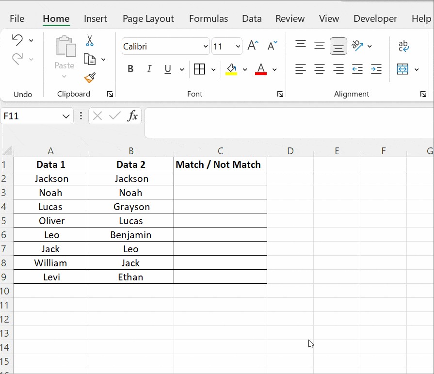
4. How To Compare Two Columns Using The IF Condition
The IF condition in Excel provides a powerful way to compare two columns and display specific results based on whether the values match. The basic formula to compare two columns is =IF(A2=B2,”Match”,” ”). This formula returns “Match” for rows where the values are identical and leaves the cell blank for rows with differing values.
Alt Text: Comparing Excel columns using IF condition to highlight matches and mismatches
To identify mismatched values, you can modify the formula to display a specific result when the IF condition is false. For instance, the formula =IF(A2=B2,”Match”,”Not a Match ”) returns “Match” for identical values and “Not a Match” for differing values.
To specifically compare two columns for differences, replace the equals sign (=) with the not-equal-to sign (<>). The formula =IF(A2<>B2,”Match”,”Not a Match ”) will return “Match” for rows where the values are different and “Not a Match” where they are the same.
5. Using The EXACT() Function For Case-Sensitive Comparisons
When comparing columns containing text, it’s often necessary to perform a case-sensitive comparison. This is where the EXACT() function comes in handy.
The EXACT() function compares two text strings and returns TRUE if they are exactly the same, including case, and FALSE otherwise. Importantly, EXACT() is case-sensitive but ignores formatting differences. The syntax is straightforward: =EXACT(text1, text2), where text1 and text2 are the two text strings you want to compare. Both arguments are required.
Consider an example where columns A and B contain the text string “Nova Scotia”.
Using the formula =IF(A2=B2, “Match”, “Mismatch”) in cell C2 would return “Match” because this comparison is case-insensitive.
However, to perform a case-sensitive comparison, use the formula =IF(EXACT(A2, B2), “Match”, “Mismatch”).
In this case, the EXACT() function first compares the text strings in A2 and B2. If they are exactly the same, including case, EXACT() returns TRUE. Otherwise, it returns FALSE. The IF function then uses this result to display either “Match” or “Mismatch” accordingly.
6. Conditional Formatting For Highlighting Differences and Similarities
Conditional formatting is a powerful tool for visually highlighting differences or similarities between two columns in Excel. To use this feature, follow these steps:
- Select the range of cells you want to format.
- Go to Home tab, then click on Conditional Formatting in the Styles group.
- Choose Highlight Cells Rules and then select Duplicate Values.
This will open a dialog box where you can specify the formatting options:
- Apply the formatting condition to the cells: You can choose either Duplicate or Unique.
- Format cells that contain: In this section, you can choose the formatting style, such as filling with color, changing the text color, or altering the cell border.
Alt Text: Excel conditional formatting options for comparing columns and highlighting duplicates and unique values.
For example, if you have two columns of names (Data1 and Data2), and you want to highlight the names that appear in both columns, select both columns, follow the steps above, and choose Duplicate. Then, choose your desired formatting option (e.g., fill with a specific color). Excel will then highlight all the names that are present in both columns.
If, instead, you want to highlight the names that are unique to each column (i.e., names that appear in only one column), follow the same steps but choose Unique instead of Duplicate.
Alt Text: Highlighting unique values in Excel using conditional formatting for data comparison.
Tip: To remove the conditional formatting, go to Conditional Formatting → Clear Rules → Clear Rules from Selected Cells.
Conditional formatting is particularly useful when you don’t want to add a third column to display the comparison results. It allows you to visually identify duplicate (matching) and unique (different) data directly within the columns. However, this method is best suited for smaller tables. For larger spreadsheets, more advanced methods may be necessary.
7. Leveraging LOOKUP Functions For Advanced Column Comparisons
The LOOKUP function family in Excel allows you to search for a specific value within a row or column and return a corresponding value from another row or column. Excel offers several LOOKUP functions, including HLOOKUP, VLOOKUP, and XLOOKUP.
- HLOOKUP (Horizontal Lookup): Searches for a value in the top row of a table and returns a value from a specified row in the same column.
- VLOOKUP (Vertical Lookup): Searches for a value in the first column of a table and returns a value from a specified column in the same row.
- XLOOKUP: A more versatile function that combines the capabilities of both HLOOKUP and VLOOKUP, allowing you to search in either rows or columns and return values from any direction.
Here’s an example of using VLOOKUP() to compare two columns in Excel:
Alt Text: Comparing Excel columns using the VLOOKUP function for data matching.
In this scenario, column A contains a list of exams taken by a student, and column B lists the subjects the student has passed. To determine which exams the student passed, you can use the VLOOKUP() function. In cell C2, enter the formula =VLOOKUP(A2, $B$2:$B$5,1,0).
Drag the formula down to apply it to all the cells in column C. The results will show the subjects the student passed, with “#N/A” indicating the subjects not cleared.
Let’s break down the formula:
- VLOOKUP(A2,..,..,..): This specifies that the function should look up the value in cell A2.
- VLOOKUP(A2, $B$2:$B$5,..,..): This indicates the range of cells (B2 to B5) to compare the value from A2 against. The dollar signs ($) create an absolute reference, ensuring that the range remains fixed when the formula is dragged down.
- VLOOKUP(A2, $B$2:$B$5,1,..): The third argument, “col_index_num,” specifies the column from which to return the value if a match is found. In this case, it’s set to 1, indicating that the value should be returned from the first column in the specified range (B2:B5).
- VLOOKUP(A2, $B$2:$B$5,1,0): The last argument is a logical value that determines whether to find an exact match (0) or an approximate match (1). In this case, 0 is used to ensure that only exact matches are returned.
8. In What Scenarios Is Comparing Columns Useful?
Comparing columns in Excel is useful in a variety of scenarios, from basic data cleaning to more complex data analysis tasks. Here are some examples:
8.1. Data Validation And Cleansing
- Identifying duplicates: Comparing columns can help you identify duplicate entries in your data, which is crucial for ensuring data accuracy and consistency.
- Checking for missing values: By comparing two columns that should contain the same data, you can quickly identify any missing values.
8.2. Financial Analysis
- Reconciling bank statements: You can compare transactions in your accounting software with your bank statements to identify any discrepancies.
- Analyzing budget vs. actual expenses: Comparing budgeted expenses with actual expenses can help you identify areas where you are over or under budget.
8.3. Sales And Marketing
- Comparing sales data across regions: Comparing sales data from different regions can help you identify top-performing areas and areas that need improvement.
- Analyzing marketing campaign performance: Comparing the results of different marketing campaigns can help you determine which strategies are most effective.
8.4. Inventory Management
- Comparing inventory levels across warehouses: Comparing inventory levels at different warehouses can help you optimize stock distribution and reduce storage costs.
- Tracking product sales: Comparing sales data with inventory levels can help you identify slow-moving products and prevent stockouts.
8.5. Human Resources
- Comparing employee data across departments: Comparing employee information across different departments can help you identify trends and ensure fair compensation practices.
- Tracking employee performance: Comparing performance data across different periods can help you identify top performers and areas where employees need improvement.
9. Frequently Asked Questions
9.1. What Is The Easiest Way To Compare Two Columns In Excel?
One of the simplest methods to compare two columns in Excel is to select both columns, then navigate to Home → Find & Select → Go To Special → Row Differences, and click OK. This will highlight the cells that do not match across the rows, making it easy to spot the differences. The matching cells will remain white, while the unmatched cells will appear in gray.
9.2. How Can I Use The IF Condition To Compare More Than Two Columns?
To compare three or more columns using the IF condition, you can use the AND or OR statements within the IF formula:
- To find matches in all cells within the same row: Use the AND statement. The formula would be =IF(AND(A2=B2, A2=C2), “Full match”, “”). This formula returns “Full match” only if the values in all three cells (A2, B2, and C2) are identical.
- To find matches in any two cells within the same row: Use the OR statement. The formula would be =IF(OR(A2=B2, B2=C2, A2=C2), “Match”, “”). This formula returns “Match” if any two of the three cells have the same value.
9.3. Can The INDEX-MATCH Function Be Used To Compare Columns?
Yes, the INDEX-MATCH function is a powerful alternative to VLOOKUP for comparing columns in Excel. It allows you to match data between two different tables and pull corresponding entries from the comparing table.
For example, you can use the MATCH() function to compare values in one column (e.g., column D) with values in another column (e.g., column A). If a match is found, the INDEX function can then pull the corresponding value from a third column (e.g., column B) and display it. If no match is found, the formula will return #N/A.
10. Conclusion: Mastering Column Comparisons in Excel
Comparing columns in Excel is a frequent and crucial task for data analysts and anyone working with spreadsheets. Excel provides multiple methods for comparing and matching data, whether within a single column, across multiple columns, or even across multiple spreadsheets. This tutorial has outlined several effective techniques for comparing two columns in Excel to find matches, highlight differences, and extract valuable insights.
Mastering LOOKUP functions, like VLOOKUP, HLOOKUP and XLOOKUP, is essential for anyone looking to enhance their Excel skills. To further expand your knowledge of Excel functions and formulas, consider exploring courses in Excel and Microsoft Office Applications. These courses offer micro-credentials upon completion, validating your expertise.
Remember, COMPARE.EDU.VN is your go-to resource for detailed comparisons and informed decision-making. Visit our website at COMPARE.EDU.VN or contact us at our Comparison Plaza: 333 Comparison Plaza, Choice City, CA 90210, United States, or via Whatsapp at +1 (626) 555-9090. Let us help you make smarter choices.
Seeking expert guidance on choosing the right software or service? compare.edu.vn provides in-depth comparisons to assist you in making informed decisions. Visit our website today to explore a wealth of resources and expert insights tailored to your needs.