The running time of algorithms can indeed be compared, and COMPARE.EDU.VN offers the perfect platform to do just that. By analyzing the efficiency and computational complexity of different algorithms, you can determine which one is most suitable for a specific task. Explore COMPARE.EDU.VN for detailed algorithmic comparisons, performance analysis, and efficiency metrics to make informed decisions.
1. Understanding Algorithm Running Time
When evaluating algorithms, running time is a crucial factor. It refers to the amount of time an algorithm takes to execute as a function of the input size. Understanding how to compare running times of algorithms helps in choosing the most efficient one for a particular task.
1.1. Why Compare Running Times?
Comparing running times is essential because it directly impacts the performance and scalability of applications. An algorithm with a faster running time can process larger datasets more quickly, leading to better user experiences and reduced computational costs.
1.2. Asymptotic Notation: Big O, Big Theta, and Big Omega
Asymptotic notation is a mathematical notation used to describe the limiting behavior of a function when the argument tends towards a particular value or infinity. In the context of algorithms, it helps in understanding how the running time grows as the input size increases.
1.2.1. Big O Notation
Big O notation (O) provides an upper bound on the growth rate of an algorithm’s running time. It describes the worst-case scenario. For example, O(n) means the running time increases linearly with the input size n.
1.2.2. Big Theta Notation
Big Theta notation (Θ) describes the average-case running time of an algorithm, providing a tight bound on the growth rate. For example, Θ(n log n) indicates that the algorithm’s running time grows proportionally to n log n.
1.2.3. Big Omega Notation
Big Omega notation (Ω) provides a lower bound on the growth rate of an algorithm’s running time. It describes the best-case scenario. For example, Ω(1) means the algorithm takes constant time, regardless of the input size.
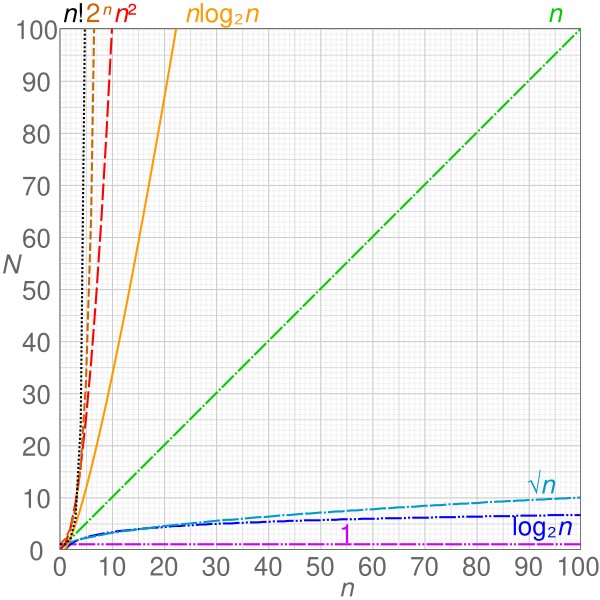 Big O Notation Chart
Alt Text: Chart comparing the growth rates of different Big O notations, including O(1), O(log n), O(n), O(n log n), O(n^2), and O(2^n), illustrating the efficiency of algorithms based on their time complexity.
2. Common Time Complexities
Different algorithms exhibit different time complexities. Understanding these complexities is crucial for comparing their running times.
2.1. Constant Time – O(1)
An algorithm with constant time complexity takes the same amount of time to execute, regardless of the input size. Examples include accessing an element in an array by its index or performing a simple arithmetic operation.
2.2. Logarithmic Time – O(log n)
Logarithmic time complexity means the running time increases logarithmically with the input size. Binary search is a classic example, where the search space is halved in each step.
2.3. Linear Time – O(n)
Linear time complexity indicates that the running time increases linearly with the input size. Examples include iterating through an array or searching for an element in an unsorted list.
2.4. Linearithmic Time – O(n log n)
Linearithmic time complexity is a combination of linear and logarithmic complexities. Merge sort and heap sort are examples of algorithms with this time complexity.
2.5. Quadratic Time – O(n^2)
Quadratic time complexity means the running time increases quadratically with the input size. Bubble sort and insertion sort are examples of algorithms with this time complexity.
2.6. Exponential Time – O(2^n)
Exponential time complexity indicates that the running time increases exponentially with the input size. These algorithms are generally inefficient for large datasets. An example is finding all subsets of a set.
2.7. Factorial Time – O(n!)
Factorial time complexity is one of the slowest-growing complexities. An example is generating all permutations of a set.
3. Methods for Comparing Algorithm Running Times
Several methods can be used to compare the running times of algorithms effectively.
3.1. Theoretical Analysis
Theoretical analysis involves analyzing the algorithm’s code to determine its time complexity using asymptotic notation. This method provides a general understanding of how the algorithm’s running time scales with the input size.
3.1.1. Identifying Dominant Operations
Identifying the dominant operations in an algorithm is crucial for theoretical analysis. These are the operations that contribute the most to the running time, especially as the input size grows.
3.1.2. Calculating Time Complexity
Calculating time complexity involves counting the number of times the dominant operations are executed as a function of the input size. This results in an expression that represents the algorithm’s time complexity.
3.2. Empirical Analysis
Empirical analysis involves running the algorithm with different input sizes and measuring its actual running time. This method provides concrete data that can be used to compare the performance of different algorithms in practice.
3.2.1. Setting Up Experiments
Setting up experiments for empirical analysis requires careful consideration of the input data, the hardware environment, and the measurement tools.
3.2.2. Measuring Execution Time
Measuring execution time accurately is essential for empirical analysis. Various tools and techniques can be used, such as timers, profilers, and system monitors.
3.3. Profiling
Profiling is a technique that involves analyzing the execution of an algorithm to identify the parts that consume the most time. This information can be used to optimize the algorithm’s performance.
3.3.1. Using Profiling Tools
Profiling tools provide detailed information about the execution of an algorithm, including the number of times each function is called, the time spent in each function, and the memory usage.
3.3.2. Identifying Bottlenecks
Identifying bottlenecks in an algorithm is crucial for optimization. These are the parts of the algorithm that consume the most time and resources.
Alt Text: Example of algorithm profiling showing CPU usage and time spent in various functions to identify performance bottlenecks and optimize code efficiency.
4. Factors Affecting Running Time
Several factors can affect the running time of an algorithm, including hardware, software, and input data.
4.1. Hardware
The hardware on which an algorithm is executed can significantly impact its running time. Factors such as CPU speed, memory capacity, and disk I/O speed can all play a role.
4.1.1. CPU Speed
A faster CPU can execute more instructions per second, leading to faster running times.
4.1.2. Memory Capacity
Sufficient memory capacity can prevent the algorithm from having to swap data to disk, which can significantly slow down execution.
4.1.3. Disk I/O Speed
Fast disk I/O speeds can improve the performance of algorithms that need to read or write large amounts of data.
4.2. Software
The software environment in which an algorithm is executed can also affect its running time. Factors such as the operating system, the programming language, and the compiler can all play a role.
4.2.1. Operating System
The operating system can affect the running time of an algorithm by managing resources such as CPU time, memory, and disk I/O.
4.2.2. Programming Language
Different programming languages have different performance characteristics. For example, compiled languages like C++ are generally faster than interpreted languages like Python.
4.2.3. Compiler
The compiler can optimize the algorithm’s code, leading to faster running times.
4.3. Input Data
The characteristics of the input data can also affect the running time of an algorithm. Factors such as the size, distribution, and structure of the data can all play a role.
4.3.1. Input Size
The input size is the most obvious factor affecting running time. Algorithms generally take longer to execute with larger input sizes.
4.3.2. Data Distribution
The distribution of the input data can also affect running time. For example, some sorting algorithms perform better with nearly sorted data than with randomly ordered data.
4.3.3. Data Structure
The data structure used to store the input data can also affect running time. For example, searching for an element in a hash table is generally faster than searching for an element in an unsorted array.
5. Case Studies: Comparing Running Times of Specific Algorithms
To illustrate the comparison of running times, let’s examine some specific algorithms.
5.1. Sorting Algorithms: Bubble Sort vs. Merge Sort
Bubble sort and merge sort are two common sorting algorithms with different time complexities.
5.1.1. Bubble Sort
Bubble sort has a time complexity of O(n^2) in the worst and average cases, and O(n) in the best case. It is generally inefficient for large datasets.
5.1.2. Merge Sort
Merge sort has a time complexity of O(n log n) in all cases. It is more efficient than bubble sort for large datasets.
5.1.3. Comparison
| Feature | Bubble Sort | Merge Sort |
|---|---|---|
| Time Complexity | O(n^2) | O(n log n) |
| Best Case | O(n) | O(n log n) |
| Space Complexity | O(1) | O(n) |
| Stability | Yes | Yes |
5.2. Searching Algorithms: Linear Search vs. Binary Search
Linear search and binary search are two common searching algorithms with different time complexities.
5.2.1. Linear Search
Linear search has a time complexity of O(n) in the worst and average cases, and O(1) in the best case. It is suitable for unsorted lists.
5.2.2. Binary Search
Binary search has a time complexity of O(log n) in the worst and average cases, and O(1) in the best case. It requires the list to be sorted.
5.2.3. Comparison
| Feature | Linear Search | Binary Search |
|---|---|---|
| Time Complexity | O(n) | O(log n) |
| Best Case | O(1) | O(1) |
| Sorted Data | No | Yes |
| Space Complexity | O(1) | O(1) |
5.3. Graph Algorithms: Depth-First Search vs. Breadth-First Search
Depth-first search (DFS) and breadth-first search (BFS) are two common graph traversal algorithms with different characteristics.
5.3.1. Depth-First Search
Depth-first search explores as far as possible along each branch before backtracking. It has a time complexity of O(V + E), where V is the number of vertices and E is the number of edges.
5.3.2. Breadth-First Search
Breadth-first search explores all the neighbors of a node before moving to the next level of neighbors. It also has a time complexity of O(V + E).
5.3.3. Comparison
| Feature | Depth-First Search | Breadth-First Search |
|---|---|---|
| Time Complexity | O(V + E) | O(V + E) |
| Space Complexity | O(V) | O(V) |
| Use Cases | Path finding, cycle detection | Shortest path, network traversal |
| Implementation | Recursive | Iterative |
Alt Text: Visual comparison of Depth-First Search (DFS) and Breadth-First Search (BFS) algorithms, illustrating their traversal paths in a graph structure and highlighting their different use cases.
6. Tools for Analyzing Algorithm Performance
Several tools are available for analyzing the performance of algorithms, including profilers, timers, and performance monitoring tools.
6.1. Profilers
Profilers provide detailed information about the execution of an algorithm, including the number of times each function is called, the time spent in each function, and the memory usage.
6.1.1. gprof
gprof is a popular profiling tool for C and C++ programs. It provides a call graph and execution time statistics for each function.
6.1.2. perf
perf is a powerful profiling tool for Linux systems. It can be used to analyze the performance of any application, including those written in C, C++, Python, and Java.
6.1.3. Java Profilers
Java profilers such as JProfiler and YourKit provide detailed information about the execution of Java programs, including CPU usage, memory usage, and thread activity.
6.2. Timers
Timers can be used to measure the execution time of an algorithm. They provide a simple way to compare the performance of different algorithms.
6.2.1. System.nanoTime() in Java
System.nanoTime() provides a high-resolution timer that can be used to measure the execution time of Java code.
6.2.2. time.perf_counter() in Python
time.perf_counter() provides a high-resolution timer that can be used to measure the execution time of Python code.
6.3. Performance Monitoring Tools
Performance monitoring tools provide real-time information about the performance of a system, including CPU usage, memory usage, disk I/O, and network traffic.
6.3.1. Task Manager in Windows
Task Manager provides real-time information about the performance of a Windows system, including CPU usage, memory usage, disk I/O, and network traffic.
6.3.2. Activity Monitor in macOS
Activity Monitor provides real-time information about the performance of a macOS system, including CPU usage, memory usage, disk I/O, and network traffic.
6.3.3. top and htop in Linux
top and htop are command-line tools that provide real-time information about the performance of a Linux system, including CPU usage, memory usage, and process activity.
7. Best Practices for Improving Algorithm Performance
Several best practices can be followed to improve the performance of algorithms.
7.1. Choosing the Right Algorithm
Choosing the right algorithm for a particular task is crucial for achieving optimal performance. Consider the time complexity, space complexity, and other characteristics of different algorithms before making a decision.
7.2. Optimizing Code
Optimizing code can significantly improve the performance of an algorithm. Techniques such as loop unrolling, inlining functions, and reducing memory allocations can all help.
7.3. Using Efficient Data Structures
Using efficient data structures can also improve the performance of an algorithm. For example, using a hash table instead of an array can significantly speed up searching operations.
7.4. Parallelization
Parallelization involves dividing an algorithm into smaller tasks that can be executed simultaneously on multiple processors. This can significantly reduce the running time of the algorithm.
7.5. Caching
Caching involves storing frequently used data in memory so that it can be accessed more quickly. This can significantly improve the performance of algorithms that access the same data repeatedly.
Alt Text: Visualization of different optimization techniques used in algorithm design, including loop optimization, data structure optimization, and parallelization, to improve overall performance.
8. The Role of COMPARE.EDU.VN in Algorithm Comparison
COMPARE.EDU.VN plays a vital role in helping users compare the running times and performance of different algorithms. By providing detailed analyses, empirical data, and expert insights, COMPARE.EDU.VN empowers users to make informed decisions about which algorithms to use for their specific needs.
8.1. Providing Detailed Analyses
COMPARE.EDU.VN offers detailed analyses of various algorithms, including their time complexity, space complexity, and other performance characteristics. This information helps users understand the strengths and weaknesses of each algorithm and choose the one that is most suitable for their task.
8.2. Offering Empirical Data
COMPARE.EDU.VN provides empirical data on the running times of different algorithms, based on experiments conducted under controlled conditions. This data allows users to compare the performance of algorithms in practice and see how they scale with different input sizes.
8.3. Expert Insights
COMPARE.EDU.VN features expert insights from leading computer scientists and software engineers. These insights provide valuable perspectives on the performance of different algorithms and help users understand the factors that can affect their running times.
9. Future Trends in Algorithm Analysis
The field of algorithm analysis is constantly evolving, with new techniques and tools being developed all the time. Some of the key trends in this field include:
9.1. Automated Algorithm Analysis
Automated algorithm analysis involves using machine learning techniques to automatically analyze the performance of algorithms. This can help to identify bottlenecks, optimize code, and choose the right algorithm for a particular task.
9.2. Real-Time Performance Monitoring
Real-time performance monitoring involves monitoring the performance of algorithms in real time, allowing users to identify and address performance issues as they arise.
9.3. Integration with Development Tools
Integration with development tools involves integrating algorithm analysis tools into the development environment, making it easier for developers to analyze the performance of their code.
10. Conclusion: Making Informed Decisions with COMPARE.EDU.VN
Comparing the running times of algorithms is essential for making informed decisions about which algorithms to use for specific tasks. By understanding the concepts of time complexity, asymptotic notation, and empirical analysis, you can effectively compare the performance of different algorithms and choose the one that is most suitable for your needs.
COMPARE.EDU.VN provides a comprehensive platform for comparing the running times and performance of various algorithms. With detailed analyses, empirical data, and expert insights, COMPARE.EDU.VN empowers users to make informed decisions and optimize their applications for maximum performance.
Are you struggling to decide which algorithm is best for your project? Visit COMPARE.EDU.VN at 333 Comparison Plaza, Choice City, CA 90210, United States, or contact us via Whatsapp at +1 (626) 555-9090 for expert guidance and detailed comparisons. Let COMPARE.EDU.VN help you make the right choice and optimize your application’s performance.
FAQ: Frequently Asked Questions
1. What is time complexity?
Time complexity is a measure of the amount of time an algorithm takes to complete, expressed as a function of the size of the input. It helps in understanding how the running time of an algorithm scales with the input size.
2. Why is it important to compare running times of algorithms?
Comparing running times is important because it helps in choosing the most efficient algorithm for a specific task, leading to better performance and scalability.
3. What is Big O notation?
Big O notation is a mathematical notation used to describe the upper bound of an algorithm’s running time. It represents the worst-case scenario and provides a general understanding of how the algorithm’s running time scales with the input size.
4. How does hardware affect the running time of an algorithm?
Hardware factors such as CPU speed, memory capacity, and disk I/O speed can significantly impact the running time of an algorithm. Faster hardware generally leads to faster execution times.
5. What are some common time complexities?
Common time complexities include O(1) (constant time), O(log n) (logarithmic time), O(n) (linear time), O(n log n) (linearithmic time), and O(n^2) (quadratic time).
6. Can empirical analysis provide more accurate results than theoretical analysis?
Empirical analysis provides concrete data based on actual execution times, which can be more accurate than theoretical analysis, especially when considering real-world factors such as hardware and software environments.
7. What tools can be used to analyze algorithm performance?
Tools such as profilers (gprof, perf), timers (System.nanoTime() in Java, time.perf_counter() in Python), and performance monitoring tools (Task Manager, Activity Monitor) can be used to analyze algorithm performance.
8. How does COMPARE.EDU.VN help in comparing algorithm running times?
compare.edu.vn provides detailed analyses, empirical data, and expert insights to help users compare the running times and performance of different algorithms, enabling informed decision-making.
9. What are some best practices for improving algorithm performance?
Best practices include choosing the right algorithm, optimizing code, using efficient data structures, parallelization, and caching.
10. What are some future trends in algorithm analysis?
Future trends include automated algorithm analysis, real-time performance monitoring, and integration with development tools.