Can Mode Be Compared to Mean: An Exhaustive Comparison?

Are you struggling to understand the nuances between mode and mean and how they influence data interpretation? COMPARE.EDU.VN offers a comprehensive guide that simplifies these statistical concepts, enabling you to make informed decisions. Explore our in-depth analysis, focusing on central tendency and data distribution, to gain clarity and enhance your analytical skills.

1. What Is the Difference Between Mode and Mean?

The mode and mean are both measures of central tendency, but they represent different aspects of a dataset. The mode is the value that appears most frequently in a dataset, while the mean is the average of all values. Understanding these differences is crucial for data analysis and interpretation.

The Mode: Represents the most frequent value.
The Mean: Represents the average value.

Understanding the distinction between these two measures can provide valuable insights into the distribution and characteristics of your data.

1.1 Understanding the Mode

The mode is the value that appears most frequently in a dataset. It is a simple and intuitive measure, especially useful for categorical data.

Definition: The value that occurs most often in a data set.
Calculation: Identify the value that appears most frequently.
Use Cases: Identifying the most popular product, the most common response in a survey, or the most frequent category in a dataset.

1.2 Understanding the Mean

The mean, also known as the average, is calculated by summing all the values in a dataset and dividing by the number of values. It is widely used due to its sensitivity to all data points.

Definition: The sum of all values divided by the number of values.
Calculation: Sum all values and divide by the total number of values.
Use Cases: Calculating average test scores, average income, or average sales.

2. When Can Mode Be Compared to Mean?

The mode and mean can be compared when analyzing the central tendency of a dataset, but their applicability depends on the data’s distribution and type. In symmetrical distributions, the mean and mode tend to be similar. However, in skewed distributions, they diverge, providing insights into the data’s asymmetry.

Symmetrical Distributions: Mean and mode are often similar.
Skewed Distributions: Mean and mode differ significantly.

2.1 Comparing Mode and Mean in Symmetrical Distributions

In a symmetrical distribution, the data is evenly distributed around the mean. In such cases, the mean and mode are typically close to each other, providing a consistent measure of central tendency.

Characteristics: Data is evenly distributed.
Relationship: Mean and mode are approximately equal.
Examples: Normal distribution, bell curve.

Symmetrical Distribution

Alt text: Symmetrical distribution histogram showing a bell curve where the mean and mode are equal and located at the center.

2.2 Comparing Mode and Mean in Skewed Distributions

In skewed distributions, the data is not evenly distributed. Skewness can be either to the left (negative skew) or to the right (positive skew). In such cases, the mean and mode can differ significantly, reflecting the skewness of the data.

Right Skew (Positive Skew): The mean is greater than the mode.
Left Skew (Negative Skew): The mean is less than the mode.

3. How to Compare Mode and Mean Effectively?

To effectively compare the mode and mean, consider the shape of the data distribution, the presence of outliers, and the type of data you are analyzing. Visual aids such as histograms and box plots can be invaluable in understanding the relationship between these measures.

Assess Data Distribution: Determine if the data is symmetrical or skewed.
Identify Outliers: Outliers can significantly affect the mean.
Use Visual Aids: Histograms and box plots provide visual context.

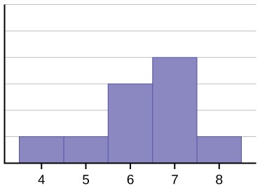
3.1 Using Histograms to Compare Mode and Mean

Histograms are graphical representations of data distribution. They allow you to visualize the frequency of different values and identify the mode. By plotting the mean on the histogram, you can easily see how it relates to the distribution and the mode.

Visualizing Frequency: Histograms show how often each value occurs.
Identifying the Mode: The highest bar represents the mode.
Comparing with the Mean: Plotting the mean on the histogram shows its position relative to the data distribution.

3.2 Using Box Plots to Compare Mode and Mean

Box plots provide a summary of the data’s distribution, including the median, quartiles, and outliers. While box plots do not directly show the mode, they help identify skewness, which influences the relationship between the mean and mode.

Summarizing Distribution: Box plots show the median, quartiles, and range.
Identifying Skewness: The position of the median relative to the box indicates skewness.
Understanding the Mean: Comparing the median to the mean (which is not shown on the box plot but can be inferred) helps understand the distribution.

4. What Are the Advantages of Comparing Mode and Mean?

Comparing the mode and mean provides a comprehensive understanding of a dataset’s central tendency and distribution. This comparison can reveal insights into the symmetry, skewness, and presence of outliers, aiding in more informed decision-making.

Comprehensive Understanding: Provides insights into central tendency and distribution.
Identifying Skewness: Reveals the asymmetry of the data.
Detecting Outliers: Highlights values that deviate significantly from the norm.

4.1 Gaining Insights into Data Symmetry

In symmetrical distributions, the mean and mode are similar, indicating a balanced dataset. This can be valuable in scenarios where consistency and predictability are important.

Balanced Data: Symmetrical distributions indicate even distribution.
Consistency: Similar mean and mode values suggest consistent data.
Predictability: Balanced data allows for more accurate predictions.

4.2 Identifying Data Skewness

Significant differences between the mean and mode indicate skewness. Understanding the direction and extent of skewness is crucial for accurate data interpretation and decision-making.

Direction of Skew: The mean is greater than the mode in right-skewed distributions, and less than the mode in left-skewed distributions.
Extent of Skew: The larger the difference between the mean and mode, the greater the skew.
Data Interpretation: Skewness affects how data should be interpreted and used for analysis.

4.3 Detecting Outliers

Outliers are extreme values that can significantly affect the mean. By comparing the mean and mode, you can identify the presence of outliers and assess their impact on the dataset.

Impact on the Mean: Outliers can pull the mean away from the typical values.
Mode Stability: The mode is generally less affected by outliers.
Assessing Impact: Comparing the mean and mode helps understand the influence of outliers.

5. What Are the Limitations of Comparing Mode and Mean?

While comparing the mode and mean is useful, it has limitations. The mode may not be unique or may not exist in some datasets, and the mean can be heavily influenced by outliers. Therefore, it is important to use these measures in conjunction with other statistical tools and techniques.

Mode Uniqueness: Datasets may have multiple modes or no mode.
Mean Sensitivity: The mean is highly sensitive to outliers.
Context Dependency: The interpretation of mode and mean depends on the context and type of data.

5.1 Issues with Mode Uniqueness

Some datasets may have multiple modes (bimodal or multimodal), making it difficult to identify a single most frequent value. In other cases, no value may appear more than once, resulting in no mode.

Bimodal Distributions: Two values appear with equal frequency.
Multimodal Distributions: More than two values appear with equal frequency.
No Mode: No value appears more than once.

5.2 Mean Sensitivity to Outliers

The mean is calculated by summing all values and dividing by the number of values, making it highly sensitive to outliers. Extreme values can disproportionately affect the mean, potentially misrepresenting the typical value.

Disproportionate Influence: Outliers can significantly skew the mean.
Misrepresentation: The mean may not accurately reflect the central tendency in the presence of outliers.
Need for Adjustment: Techniques like trimming or winsorizing may be necessary to reduce the impact of outliers.

5.3 Contextual Limitations

The interpretation of mode and mean depends on the context and type of data being analyzed. For example, in some cases, the mode may be more relevant than the mean, while in others, the opposite is true.

Data Type: The type of data (e.g., categorical, numerical) influences the relevance of mode and mean.
Research Question: The specific question being addressed determines which measure is more appropriate.
Domain Knowledge: Understanding the context and domain is crucial for accurate interpretation.

6. How Is the Mode Calculated?

Calculating the mode involves identifying the value that appears most frequently in a dataset. This process is straightforward for small datasets but can be more complex for larger datasets.

Manual Calculation: For small datasets, simply count the occurrences of each value.
Software Tools: For larger datasets, use software like Excel, R, or Python.
Frequency Tables: Create frequency tables to organize and count the data.

6.1 Manual Calculation of the Mode

For small datasets, manual calculation of the mode is feasible. This involves listing each unique value and counting its occurrences. The value with the highest count is the mode.

List Unique Values: Identify all unique values in the dataset.
Count Occurrences: Count how many times each value appears.
Identify the Mode: The value with the highest count is the mode.

6.2 Using Software Tools to Calculate the Mode

For larger datasets, using software tools is more efficient. Excel, R, and Python offer functions to calculate the mode quickly and accurately.

Excel: Use the MODE function.
R: Use the Mode function from the DescTools package.
Python: Use the mode function from the statistics module.

6.3 Creating Frequency Tables to Find the Mode

Frequency tables organize data by listing each unique value and its frequency. This makes it easier to identify the mode, especially in larger datasets.

List Unique Values: Create a column listing each unique value.
Count Frequencies: Create a column listing the frequency of each value.
Identify the Mode: The value with the highest frequency is the mode.

7. How Is the Mean Calculated?

Calculating the mean involves summing all the values in a dataset and dividing by the number of values. This is a fundamental statistical calculation widely used in various fields.

Sum All Values: Add up all the values in the dataset.
Count the Number of Values: Determine the total number of values.
Divide the Sum by the Count: The result is the mean.

7.1 Manual Calculation of the Mean

For small datasets, the mean can be easily calculated manually. This involves adding all the numbers together and dividing by the count of those numbers.

Example: For the dataset [2, 4, 6, 8], the sum is 2 + 4 + 6 + 8 = 20. There are 4 numbers, so the mean is 20 / 4 = 5.

7.2 Using Software Tools to Calculate the Mean

For larger datasets, software tools are more efficient. Excel, R, and Python provide functions to calculate the mean quickly.

Excel: Use the AVERAGE function.
R: Use the mean() function.
Python: Use the mean() function from the statistics module or NumPy library.

7.3 Weighted Mean Calculation

In some cases, each value in a dataset may have a different weight or importance. The weighted mean accounts for these differences by multiplying each value by its weight before summing and dividing by the sum of the weights.

Formula: Weighted Mean = Σ(value * weight) / Σ(weight)
Example: If you have test scores of 80, 90, and 70 with weights of 0.3, 0.4, and 0.3 respectively, the weighted mean is (80 0.3 + 90 0.4 + 70 * 0.3) / (0.3 + 0.4 + 0.3) = 80.

8. Real-World Applications of Comparing Mode and Mean

Comparing the mode and mean has numerous real-world applications across various fields, including business, healthcare, and education.

Business: Analyzing sales data to identify popular products and average sales values.
Healthcare: Examining patient data to determine common conditions and average recovery times.
Education: Evaluating student performance to identify common scores and average grades.

8.1 Business Applications

In business, comparing the mode and mean can provide valuable insights into customer behavior, sales trends, and market performance.

Sales Analysis: Identify the most frequently sold product (mode) and the average sales value (mean).
Market Research: Determine the most common customer demographics (mode) and the average customer spending (mean).
Inventory Management: Track the most popular items (mode) and the average inventory levels (mean).

8.2 Healthcare Applications

In healthcare, comparing the mode and mean can help analyze patient data, identify common health issues, and evaluate treatment effectiveness.

Patient Demographics: Determine the most common age group (mode) and the average age of patients (mean).
Treatment Outcomes: Identify the most frequent treatment outcome (mode) and the average recovery time (mean).
Disease Prevalence: Track the most common diseases (mode) and the average number of cases (mean).

8.3 Education Applications

In education, comparing the mode and mean can provide insights into student performance, identify common scores, and evaluate the effectiveness of teaching methods.

Test Scores: Identify the most frequent score (mode) and the average score (mean).
Student Demographics: Determine the most common grade level (mode) and the average age of students (mean).
Course Evaluation: Assess the most common feedback (mode) and the average satisfaction rating (mean).

9. Case Studies on Comparing Mode and Mean

Examining specific case studies can further illustrate the practical applications and benefits of comparing the mode and mean.

Case Study 1: Retail Sales Analysis: Comparing the mode and mean of sales data to optimize inventory and marketing strategies.
Case Study 2: Healthcare Data Analysis: Analyzing patient data to improve treatment protocols and resource allocation.
Case Study 3: Educational Performance Evaluation: Evaluating student performance data to enhance teaching methods and curriculum development.

9.1 Case Study 1: Retail Sales Analysis

A retail company analyzed its sales data and found that the mode for product sales was a specific brand of coffee, while the mean sales value was relatively low. This indicated that while this brand was popular, customers were buying it in small quantities. The company then implemented a promotion to encourage larger purchases, which increased the average sales value and overall revenue.

Initial Finding: High mode, low mean for a specific product.
Action Taken: Implemented a promotion to encourage larger purchases.
Outcome: Increased average sales value and overall revenue.

9.2 Case Study 2: Healthcare Data Analysis

A hospital analyzed patient data and found that the mode for patient age was in the 60-65 age range, while the mean age was slightly higher due to a few elderly patients. This information helped the hospital tailor its services to the needs of the most common age group while also addressing the specific health concerns of older patients.

Initial Finding: Mode in the 60-65 age range, slightly higher mean.
Action Taken: Tailored services to the needs of the most common age group.
Outcome: Improved patient care and resource allocation.

9.3 Case Study 3: Educational Performance Evaluation

A school district analyzed student test scores and found that the mode was a score of 75, while the mean was slightly lower due to some students performing poorly. The district then implemented targeted interventions for struggling students, which improved their scores and increased the overall mean performance.

Initial Finding: Mode of 75, slightly lower mean.
Action Taken: Implemented targeted interventions for struggling students.
Outcome: Improved student scores and increased overall mean performance.

10. Frequently Asked Questions (FAQs) About Comparing Mode and Mean

10.1 What does it mean if the mean and mode are the same?

If the mean and mode are the same, the data distribution is likely symmetrical, indicating a balanced dataset where the average value is also the most frequent value.

10.2 When should I use the mode instead of the mean?

Use the mode when you want to identify the most frequent value in a dataset, especially for categorical data or when the data is highly skewed.

10.3 Can a dataset have more than one mode?

Yes, a dataset can have more than one mode (bimodal or multimodal) if two or more values appear with equal frequency.

10.4 How do outliers affect the mean and mode?

Outliers can significantly affect the mean by pulling it away from the typical values, while the mode is generally less affected by outliers.

10.5 What is skewness, and how does it relate to the mean and mode?

Skewness refers to the asymmetry of a data distribution. In right-skewed distributions, the mean is greater than the mode, while in left-skewed distributions, the mean is less than the mode.

10.6 Is the mean always the best measure of central tendency?

No, the mean is not always the best measure of central tendency, especially when the data is skewed or contains outliers. In such cases, the median or mode may be more appropriate.

10.7 How can I visualize the relationship between the mean and mode?

Use histograms and box plots to visualize the relationship between the mean and mode. Histograms show the frequency of different values, while box plots summarize the distribution and highlight skewness.

10.8 What software can I use to calculate the mean and mode?

You can use software like Excel, R, and Python to calculate the mean and mode quickly and accurately.

10.9 How do I calculate the weighted mean?

The weighted mean is calculated by multiplying each value by its weight, summing the results, and dividing by the sum of the weights.

10.10 Why is it important to compare the mean and mode?

Comparing the mean and mode provides a comprehensive understanding of a dataset’s central tendency and distribution, helping you make more informed decisions and avoid misinterpretations.

11. Conclusion: Making Informed Decisions with Mode and Mean Comparison

Comparing the mode and mean provides a comprehensive understanding of a dataset’s central tendency and distribution. While the mean offers an average value influenced by all data points, the mode highlights the most frequent value. Understanding their differences and comparing them effectively is essential for accurate data interpretation and informed decision-making. By considering the shape of the data distribution, the presence of outliers, and the type of data you are analyzing, you can leverage these measures to gain valuable insights.

For more detailed comparisons and data analysis tools, visit COMPARE.EDU.VN. Our platform provides in-depth resources to help you make data-driven decisions with confidence. Whether you’re analyzing sales data, healthcare metrics, or educational performance, COMPARE.EDU.VN offers the insights you need. Contact us at 333 Comparison Plaza, Choice City, CA 90210, United States or reach out via WhatsApp at +1 (626) 555-9090.

Ready to make smarter choices? Explore COMPARE.EDU.VN today and unlock the power of comprehensive data comparison!

12. Call to Action

Are you ready to make data-driven decisions with confidence? Visit COMPARE.EDU.VN to explore our comprehensive comparisons and analysis tools. Whether you’re comparing products, services, or ideas, our platform provides the insights you need to make the best choices. Explore now and start making smarter decisions today!

Alt text: Data comparison interface on COMPARE.EDU.VN showing detailed analysis of different metrics, emphasizing data-driven decision-making.

Address: 333 Comparison Plaza, Choice City, CA 90210, United States. Whatsapp: +1 (626) 555-9090. Website: COMPARE.EDU.VN. Let compare.edu.vn be your guide in navigating the complexities of data analysis and decision-making.