Mastering Excel: How to Compare Two Columns for Data Analysis

In the world of data analysis, Microsoft Excel remains an indispensable tool. Whether you’re managing sales figures, tracking inventory, or analyzing research data, Excel’s spreadsheets are crucial for organization and insight. A common task for anyone working with Excel is comparing two columns of data. This might seem straightforward for small datasets, but when you’re dealing with large spreadsheets, manual comparison becomes incredibly time-consuming and prone to error.

Imagine sifting through thousands of rows, trying to identify matching or unique entries between two columns. Without the right techniques, you could spend hours on a task that Excel can handle efficiently in minutes. This is where understanding how to effectively Compare Two Columns In Excel becomes essential.

This comprehensive guide will walk you through various methods to compare two columns in Excel, from simple formulas to more advanced features like conditional formatting and lookup functions. We’ll equip you with the skills to quickly identify matches, find differences, and highlight unique or duplicate values. Whether you are looking to reconcile data, find discrepancies, or simply understand the relationships within your information, mastering these techniques will significantly enhance your data analysis workflow and save you valuable time. Let’s explore how to confidently compare two columns in Excel and unlock deeper insights from your data.

Why Compare Two Columns in Excel? Unlocking Data Insights

Excel’s power lies in its ability to transform raw data into actionable information. Comparing two columns is a fundamental operation that underpins many data analysis tasks. Here’s why it’s so useful:

• Data Validation and Cleansing: Ensure data consistency across different datasets. For example, compare a list of customer emails against a marketing campaign list to identify discrepancies or missing entries.
• Identifying Duplicates and Unique Entries: Quickly pinpoint duplicate entries for data cleansing or highlight unique items for specific analysis, such as finding new customers in a recent sales list compared to a master customer database.
• Reconciling Data Sets: Compare financial records, inventory lists, or sales reports from different periods to reconcile data and identify discrepancies, errors, or areas needing attention.
• Tracking Changes Over Time: Compare datasets from different time points to analyze trends, growth, or decline. For instance, compare sales figures from this month to last month to track performance.
• Finding Matching Records: Identify records that exist in both columns, useful for merging datasets or verifying information across different sources.

Manually performing these comparisons on large datasets is not only tedious but also highly inefficient. Excel offers several built-in tools and formulas that automate this process, making it faster, more accurate, and less prone to human error. By learning these methods to compare two columns in Excel, you gain a powerful advantage in data analysis and decision-making.

Methods to Compare Two Columns in Excel: A Step-by-Step Guide

Excel provides a range of methods to compare two columns, each suited to different needs and levels of complexity. Here, we’ll explore the most effective techniques, starting from simple operators to more advanced functions.

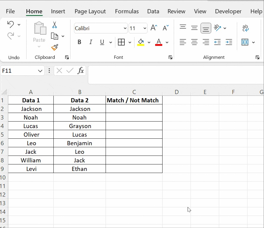
1. Row-by-Row Comparison with the Equals Operator (=)

The most basic method to compare two columns in Excel is a row-by-row comparison using the equals operator (=). This method is ideal for a quick visual check and identifying exact matches in corresponding rows.

Steps:

1. Choose a helper column: Select an empty column adjacent to the columns you want to compare (e.g., column C if you are comparing columns A and B).
2. Enter the formula: In the first cell of the helper column (e.g., C2), enter the formula =A2=B2. This formula compares the value in cell A2 with the value in cell B2.
3. Press Enter: Excel will return TRUE if the values in A2 and B2 are identical, and FALSE if they are different.
4. Drag the fill handle: Click and drag the small square at the bottom-right corner of cell C2 down to apply the formula to the rest of the rows in your data.

Now, column C will display TRUE or FALSE for each row, indicating whether the values in columns A and B match in that row. You can easily scan down column C to visually identify rows where the columns differ.

2. Conditional Comparison with the IF Function

While the equals operator shows TRUE or FALSE, you might want more descriptive results like “Match” or “Mismatch”. The IF function allows you to customize the output when you compare two columns in Excel.

Steps:

1. Choose a helper column: Again, select an empty column.
2. Enter the IF formula for matches: In the first cell of the helper column (e.g., C2), enter the formula =IF(A2=B2,"Match","Mismatch"). This formula checks if A2 equals B2. If TRUE, it returns “Match”; if FALSE, it returns “Mismatch”.
3. Press Enter and drag the fill handle: Apply the formula to the remaining rows as before.

Formula variations:

• To show “Match” and leave blanks for mismatches: =IF(A2=B2,"Match","")
• To find differences instead of matches (using the not-equal-to operator <>): =IF(A2<>B2,"Different","Same") or =IF(A2<>B2,"Mismatch","")

The IF function provides more user-friendly results when you compare two columns in Excel, making it easier to interpret the comparison outcomes at a glance.

3. Case-Sensitive Comparison with the EXACT Function

The equals operator and IF function are case-insensitive, meaning they treat “Apple” and “apple” as the same. If you need a case-sensitive comparison, use the EXACT() function.

Steps:

1. Choose a helper column.
2. Enter the EXACT formula within an IF function: In the first cell (e.g., C2), use the formula =IF(EXACT(A2,B2),"Match (Case Sensitive)","Mismatch"). The EXACT(A2,B2) function returns TRUE only if A2 and B2 are exactly the same, including case.
3. Press Enter and drag the fill handle.

Understanding EXACT Function Syntax:

The syntax for the EXACT function is =EXACT(text1, text2), where:

• text1: The first text string to compare.
• text2: The second text string to compare.

The EXACT function is crucial when case sensitivity is important in your data comparison, ensuring accurate matching of text values.

4. Highlighting Matches or Differences with Conditional Formatting

For visually highlighting matches or differences directly within your columns, conditional formatting is a powerful feature when you compare two columns in Excel. This method avoids adding a helper column and directly formats the cells based on your comparison criteria.

Steps:

1. Select the data range: Select the two columns you want to compare (e.g., columns A and B).

2. Go to Conditional Formatting: On the Home tab, in the Styles group, click “Conditional Formatting.”

3. Choose “Highlight Cells Rules” and then “Duplicate Values…” (Even though we might be looking for unique values too, this option allows customization for both).

4. In the “Duplicate Values” dialog box:

   • To highlight values present in both columns (matches):

     • In the dropdown next to the first label, ensure “Duplicate” is selected.
     • Choose your desired formatting style (e.g., fill color, text color).
     • Click “OK.”

   • To highlight values unique to each column (differences):

     • In the dropdown next to the first label, select “Unique.”
     • Choose a different formatting style to distinguish unique values (e.g., different fill color).
     • Click “OK.”

By using “Duplicate Values” and “Unique Values” in conditional formatting, you can visually distinguish matching and unique entries between your two columns directly in the spreadsheet, making it easy to spot patterns and discrepancies.

Clearing Conditional Formatting: To remove the applied formatting, go to Conditional Formatting → Clear Rules → Clear Rules from Entire Sheet or Clear Rules from Selected Cells.

Conditional formatting is excellent for visual analysis, especially for smaller to medium-sized datasets. For very large spreadsheets, formulas and lookup functions might offer more flexibility and performance.

5. Using Lookup Functions for Advanced Comparison (VLOOKUP)

For more complex comparisons, especially when you need to check if values from one column exist in another column (regardless of row order), lookup functions like VLOOKUP are invaluable when you compare two columns in Excel. VLOOKUP is particularly useful when you want to see if values in one column are present in another and potentially retrieve related information.

Scenario: Imagine you have two columns: Column A lists product IDs sold this month, and Column B is a master list of all product IDs. You want to identify which sold product IDs are in the master list and which are not.

Steps using VLOOKUP:

1. Choose a helper column.

2. Enter the VLOOKUP formula: In the first cell of the helper column (e.g., C2), enter the formula =VLOOKUP(A2,$B$2:$B$100,1,FALSE). Let’s break down this formula:

   • VLOOKUP(A2,...: This tells Excel to look up the value in cell A2.
   • $B$2:$B$100,...: This is the lookup range – the master list of product IDs in column B (from row 2 to 100 – adjust the range to fit your data). The $ signs create absolute references, so this range stays fixed when you drag the formula down.
   • ,1,...: This specifies that if a match is found, VLOOKUP should return the value from the first column of the lookup range (which is column B itself in this case).
   • ,FALSE): This ensures an exact match is found. We want to find only product IDs that are exactly the same.

3. Press Enter and drag the fill handle.

Interpreting VLOOKUP Results:

• If VLOOKUP finds a match, it will return the matching value from column B (the product ID itself).
• If VLOOKUP does not find a match, it will return #N/A.

You can then use ISNA() function along with IF to make the result more user-friendly. For example:

=IF(ISNA(VLOOKUP(A2,$B$2:$B$100,1,FALSE)),"Not Found in Master List","Found in Master List")

This formula will return “Not Found in Master List” if the product ID from column A is not in column B, and “Found in Master List” if it is.

Other Lookup Functions: While VLOOKUP is commonly used, other lookup functions like XLOOKUP (more versatile and modern) and INDEX-MATCH (more flexible for complex lookups) can also be used for comparing two columns in Excel in various scenarios.

Frequently Asked Questions about Comparing Columns in Excel

1. How can I quickly highlight row differences across two columns without formulas?

Excel’s “Go To Special” feature provides a quick way to highlight row differences.

• Select your data: Select both columns you want to compare.
• Go to “Go To Special”: Press Ctrl + G (or F5) to open the “Go To” dialog, then click “Special…”
• Choose “Row differences”: In the “Go To Special” dialog, select “Row differences” and click “OK.”

Excel will select cells that are different from the corresponding cell in the row in the first selected column. The unmatched cells will be highlighted in gray, while matching cells will appear white.

2. Can I compare more than two columns at once for matches?

Yes, you can compare multiple columns using formulas.

• For checking if all cells in a row across multiple columns are the same: Use the AND function within an IF statement. For example, to check if cells A2, B2, and C2 are all equal, use: =IF(AND(A2=B2, A2=C2), "Full Match", "")

• For checking if at least any two cells in a row across multiple columns are the same: Use the OR function within an IF statement. For example, to check if at least two of the cells A2, B2, or C2 are equal, use: =IF(OR(A2=B2, B2=C2, A2=C2), "Match", "")

3. Is it possible to compare columns in two different Excel sheets or workbooks?

Absolutely! When using formulas like VLOOKUP or the equals operator, you can reference cells in other sheets or even other open workbooks.

• Referencing cells in another sheet: When writing your formula, simply click on the other sheet and select the cells or range you need. Excel will automatically add the sheet name to your formula (e.g., 'Sheet2'!A2).
• Referencing cells in another workbook: If the other workbook is open, you can reference it similarly. Excel will include the workbook name in square brackets in your formula (e.g., '[Workbook2.xlsx]Sheet1'!B2:B100).

Conclusion: Streamlining Data Analysis by Comparing Columns in Excel

Mastering the techniques to compare two columns in Excel is a fundamental skill for anyone working with data. Whether you need to identify duplicates, reconcile datasets, or simply understand the differences between lists, Excel offers a variety of powerful tools to streamline your workflow. From basic operators and IF statements to conditional formatting and lookup functions like VLOOKUP, you now have a toolkit to efficiently analyze and compare data within your spreadsheets.

By applying these methods, you can save significant time, reduce errors, and gain deeper insights from your data. Continue practicing these techniques to enhance your Excel proficiency and become a more effective data analyst. Explore further Excel’s capabilities, including advanced formulas and data analysis features, to unlock even more potential in your data handling tasks.