Comparing maps and spatial datasets objectively can be challenging, especially when dealing with discrepancies like positional shifts, shape changes, or feature variations. This article outlines a robust method to Compare Maps by quantifying these differences using the Euclidean distance transform. It’s important to note that this approach focuses on measuring discrepancies and does not determine data quality, as “better” data is subjective and depends on the intended use.
Understanding Euclidean Distance Transform in Map Comparison
The foundation of this comparison method is the Euclidean distance transform (EDT). Imagine each map dataset as a collection of points representing geographical features. Let’s denote these datasets as ‘B’ (blue features) and ‘R’ (red features).
For every point within the map area, the EDT calculates the shortest Euclidean distance to the nearest feature in a given dataset. Visually, this transform creates a surface where the height at any point represents its proximity to the features. Points directly on features have zero height (valleys), and the surface rises with a 1:1 slope as you move away. Crucially, the EDT retains all spatial information of the dataset, making it ideal for quantitative analysis.
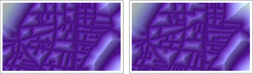
Figure 1: Distance transforms of dataset B (left) and dataset R (right) shown in pseudo-relief.
Overlaying Distance Transforms for Map Comparison
To compare maps B and R, we overlay each dataset with the EDT of the other. This means we take dataset B and color-code its features based on their distances to the nearest features in dataset R’s EDT, and vice versa for dataset R in relation to dataset B’s EDT.
Figure 2: Datasets B and R overlaid with the distance transform of the other, distance values represented by color gradients from blue (near 0) to red (far).
These overlay maps visually highlight discrepancies. For example, in the left map, features of dataset B are colored to emphasize those located far from dataset R. Both maps are essential for a comprehensive map comparison, as each reveals features that are spatially distant from the other dataset.
For enhanced visual interpretation, especially on complex maps, blurring the color-coded distance layer can improve clarity.
Figure 3: Blurred distance overlay maps for visual assessment. Note: Color scales are independent in each map, representing the full distance range within that map.
Statistical Analysis of Map Differences
The true power of this map comparison technique lies in its potential for statistical analysis. By representing the distance transforms and overlays as raster data, we can extract both local and global statistics to quantify spatial discrepancies. We can, for instance, analyze the frequency distribution of distances exceeding a certain threshold to focus on significant deviations.
Figure 4: Histograms showing distance distributions for datasets B (blue) and R (red), highlighting distances greater than three pixels. (Logarithmic horizontal axis).
As illustrated in Figure 4, these histograms reveal that blue features are more likely to be distant from red features than vice versa. This is evident from the higher blue bars extending to greater distances. A wide range of descriptive statistics can be applied to these raster datasets, allowing for detailed quantification of differences between maps, either across the entire area or within specific zones of interest.
Implementation in GIS Software for Map Comparison
Implementing this map comparison method is straightforward in most GIS software. Standard GIS platforms offer Euclidean distance transform tools (e.g., “Euclidean Distance” in ArcGIS, “r.grow.distance” in GRASS GIS) and raster overlay functionalities needed for this analysis. Blurring can be achieved using neighborhood mean or kernel convolution filters, commonly available in image processing software. While advanced statistical analysis might require exporting raster data to specialized software like R or Mathematica, the core map comparison process is readily accessible within standard GIS workflows.
By leveraging the Euclidean distance transform and overlay techniques, we can achieve a more objective and quantifiable approach to compare maps and understand the spatial discrepancies between different datasets. This method provides valuable insights for data quality assessment, change detection, and various spatial analysis applications.