Microsoft Excel is a powerful tool for data analysis, and a common task for users is to Compare Excel 2 Columns. Whether you’re auditing data, merging lists, or cleaning up spreadsheets, knowing how to effectively compare columns is essential. This guide will explore various methods to compare two columns in Excel to identify both matches and differences, enhancing your data handling skills.
Row-by-Row Comparison of Two Columns in Excel
Frequently, when working with Excel, you need to compare data on a row-by-row basis. This is where formulas come in handy, especially the versatile IF function. Let’s look at how to use it.
Example 1: Identifying Matches and Differences in the Same Row
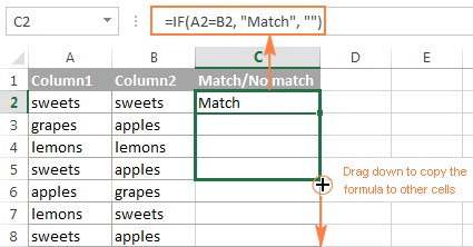
To begin, let’s compare two columns, say column A and column B, on a row-by-row basis to see if the entries in each row match or differ. You can achieve this with a simple IF formula. Enter this formula in a new column, say column C, in the first row of your data (e.g., C2 if your data starts from row 2), and then drag the fill handle down to apply it to all rows.
Formula for Identifying Matches
To specifically find rows where the content in column A and column B are identical, use the following formula:
=IF(A2=B2,"Match","")
This formula checks if the value in cell A2 is equal to the value in cell B2. If they are the same, it returns “Match”; otherwise, it returns an empty string.
Formula for Spotting Differences
Conversely, to pinpoint rows where the values in column A and column B are different, just adjust the operator to ‘<>’ (not equal to):
=IF(A2<>B2,"No match","")
This formula will return “No match” if A2 is not equal to B2, and an empty string if they are the same.
Combining Matches and Differences in One Formula
For a comprehensive view, you can combine both match and difference results in a single formula:
=IF(A2=B2,"Match","No match")
Or, alternatively:
=IF(A2<>B2,"No match","Match")
The results will clearly show matches and non-matches across your columns.
These formulas are robust and work seamlessly with numbers, dates, times, and text strings.
Tip: For an alternative to formulas, Excel’s Advanced Filter can also compare columns row-by-row. It’s especially useful for filtering and displaying matches or differences.
Example 2: Case-Sensitive Comparison for Exact Matches
The IF formulas discussed above perform case-insensitive comparisons, meaning “Apple” and “apple” are treated as matches. If you need a case-sensitive comparison, the EXACT function is your solution.
For case-sensitive matches:
=IF(EXACT(A2, B2), "Match", "")
This formula uses EXACT to compare A2 and B2. EXACT returns TRUE only if the cells are exactly the same, including case, and FALSE otherwise. The IF function then outputs “Match” for TRUE and an empty string for FALSE.
For case-sensitive differences:
=IF(EXACT(A2, B2), "Match", "Unique")
This variation outputs “Match” for exact matches and “Unique” for differences, including case differences.
Comparing Multiple Columns for Row-Based Matches
Excel’s capabilities extend to comparing more than two columns simultaneously. Here’s how to check for matches across multiple columns in each row.
Example 1: Finding Matches Across All Cells in a Row
If you have several columns and need to identify rows where all cells contain identical values, you can use a combination of IF and AND functions. For three columns (A, B, and C):
=IF(AND(A2=B2, A2=C2), "Full match", "")
For a larger number of columns, using COUNTIF can be more efficient. For example, to compare 5 columns (A to E):
=IF(COUNTIF($A2:$E2, $A2)=5, "Full match", "")
Here, COUNTIF($A2:$E2, $A2) counts how many cells in the range A2:E2 are equal to A2. If this count equals 5 (the total number of columns being compared), it signifies a full match across the row.
Example 2: Identifying Matches in Any Two Cells Within a Row
Sometimes, you might need to find rows where at least two cells match, regardless of which columns they are in. For three columns, use the OR function within an IF statement:
=IF(OR(A2=B2, B2=C2, A2=C2), "Match", "")
For a greater number of columns, summing COUNTIF functions provides a scalable solution. This approach checks each column against the subsequent columns to find any pair of matches within the row. For instance, with columns A, B, C, and D:
=IF(COUNTIF(B2:D2,A2)+COUNTIF(C2:D2,B2)+(C2=D2)=0,"Unique","Match")
This formula checks for matches between A and B, A and C, A and D, B and C, B and D, and C and D. If no matches are found (sum is 0), it marks the row as “Unique”; otherwise, it indicates a “Match”.
Comparing Two Columns for Matches and Differences Across Lists
When you need to compare two entire columns or lists to find values that are present in one but not the other, Excel offers effective techniques.
A robust method involves using COUNTIF within an IF formula. To find values in column A that are not present in column B, use:
=IF(COUNTIF($B:$B, $A2)=0, "No match in B", "")
This formula counts how many times the value from A2 appears in the entire column B. If the count is 0, it means the value is not found in column B, and the formula returns “No match in B”.
Tip: For large datasets, instead of referencing entire columns like $B:$B, specify a range (e.g., $B2:$B1000) to improve formula performance.
Alternative formulas using ISERROR and MATCH, or array formulas with SUM, can also achieve similar results, offering flexibility depending on your preference and Excel proficiency.
To identify both matches and differences, you can easily modify the formula:
=IF(COUNTIF($B:$B, $A2)=0, "No match in B", "Match in B")
Extracting Matches from Two Lists in Excel
Beyond just identifying matches, you might need to pull the matching entries from one list based on another. Excel’s VLOOKUP, INDEX MATCH, and XLOOKUP functions are designed for this purpose.
For example, to compare product names in column D against names in column A and retrieve corresponding sales figures from column B for matches, use:
VLOOKUP:
=VLOOKUP(D2, $A$2:$B$6, 2, FALSE)
INDEX MATCH:
=INDEX($B$2:$B$6, MATCH($D2, $A$2:$A$6, 0))
XLOOKUP (Excel 2021 and Microsoft 365):
=XLOOKUP(D2, $A$2:$A$6, $B$2:$B$6)
These formulas search for the value in D2 within the range A2:A6. If a match is found, they return the corresponding value from the second column (sales figures in column B) of the lookup range. If no match is found, they return a #N/A error.
Visual Comparison: Highlighting Matches and Differences
Conditional formatting in Excel allows you to visually highlight matches and differences, making it easier to identify them at a glance.
Example 1: Highlighting Row-by-Row Matches and Differences
To highlight cells in column A that match or differ from column B in the same row:
- Select the range in column A you want to format.
- Go to Home > Conditional Formatting > New Rule > Use a formula to determine which cells to format.
- For highlighting matches, use the formula
=$B2=$A2. - For highlighting differences, use the formula
=$B2<>$A2. - Choose your desired formatting and apply.
Remember to adjust the cell references (like $B2 and $A2) to match the starting row of your data.
Example 2: Highlighting Unique Entries in Two Lists
To highlight entries unique to each of two lists (e.g., List 1 in column A and List 2 in column C):
For unique values in List 1 (column A), apply conditional formatting with the formula:
=COUNTIF($C$2:$C$5, $A2)=0
For unique values in List 2 (column C), apply a rule with:
=COUNTIF($A$2:$A$6, $C2)=0
Example 3: Highlighting Matches Between Two Columns
To highlight values that are present in both columns (duplicates), adjust the COUNTIF formulas to check for counts greater than zero:
For matches in List 1 (column A):
=COUNTIF($C$2:$C$5, $A2)>0
For matches in List 2 (column C):
=COUNTIF($A$2:$A$6, $C2)>0
Highlighting Row Matches and Differences Across Multiple Columns
When comparing multiple columns row-by-row, conditional formatting remains effective for highlighting matches, while the “Go To Special” feature is a quick way to spot differences.
Example 1: Highlighting Rows with Matches Across Multiple Columns
To highlight rows where all columns have identical values:
Using AND function:
=AND($A2=$B2, $A2=$C2)
Using COUNTIF function:
=COUNTIF($A2:$C2, $A2)=3 (where 3 is the number of columns)
Apply these formulas in conditional formatting to highlight entire rows that meet the criteria.
Example 2: Highlighting Row Differences in Multiple Columns
To quickly highlight cells with different values in each row using “Go To Special”:
- Select the range of columns to compare.
- Go to Home > Editing > Find & Select > Go To Special.
- Choose “Row differences” and click OK.
- Excel will select cells that differ from the comparison cell in each row. You can then apply fill color to highlight these differences.
Comparing Two Individual Cells
Comparing two cells is a simplified version of row-by-row column comparison. Use simple IF formulas:
For matches between cell A1 and C1:
=IF(A1=C1, "Match", "")
For differences between cell A1 and C1:
=IF(A1<>C1, "Difference", "")
Formula-Free Column Comparison with Ablebits Tool
For users seeking a more streamlined, formula-free approach, the Compare Two Tables tool within Ablebits Ultimate Suite offers a powerful alternative. This add-in simplifies comparing two lists or tables by any number of columns, identifying and highlighting matches and differences.
To use the tool:
- Click Compare Tables under the Ablebits Data tab.
- Select your first list/column (Table 1).
- Select your second list/column (Table 2).
- Choose to find “Duplicate values” (matches) or “Unique values” (differences).
- Select the columns for comparison.
- Choose to highlight results or identify them in a “Status” column.
The tool provides immediate visual or textual results, enhancing efficiency in data comparison tasks.
Conclusion
Comparing two columns in Excel is a fundamental data analysis task, and Excel provides a range of tools from simple formulas to advanced features like conditional formatting and add-ins. Whether you need to compare row by row, identify list differences, or visually highlight results, Excel offers solutions to effectively compare excel 2 columns and manage your data efficiently.
Downloads
Compare Excel Lists – examples (.xlsx file)
Ultimate Suite – trial version (.exe file)