Compare Data in 2 Excel Sheets: Essential Techniques for Deep Analysis

When working with data, especially in environments reliant on spreadsheets, the need to Compare Data In 2 Excel Sheets arises frequently. Whether you are auditing financial records, reconciling inventory lists, or simply tracking changes across different versions of a report, effectively comparing Excel sheets is crucial. Identifying discrepancies, understanding modifications, and ensuring data integrity are all essential for informed decision-making and operational accuracy.

Imagine you have two versions of a sales report, each residing in a separate Excel sheet. Quickly discerning which products have shifted in performance, pinpointing new entries, or understanding pricing adjustments becomes paramount. Beyond simple reports, comparing Excel sheets can be vital for detecting broken links within workbooks, uncovering duplicate entries that skew analysis, identifying inconsistencies in formulas that lead to erroneous calculations, or flagging formatting variations that impact readability and presentation.

This guide explores a comprehensive range of methods to compare data in 2 Excel sheets, moving from straightforward visual techniques to more sophisticated, automated solutions. We will delve into native Excel functionalities and also introduce powerful third-party tools designed to streamline and enhance your data comparison tasks. By mastering these techniques, you’ll significantly improve your efficiency and accuracy when working with comparative data in Excel.

1. Side-by-Side Viewing: A Visual Approach to Compare Excel Sheets

For datasets that are manageable in size and when a quick, visual check is sufficient, leveraging Excel’s “View Side by Side” mode offers a remarkably simple solution to compare data in 2 Excel sheets. This feature allows you to arrange two Excel windows directly next to each other, facilitating a direct visual scan for differences. This method is applicable whether you’re comparing two distinct Excel workbooks or two different sheets within the same workbook.

1.1. How to Compare Two Excel Workbooks in Side-by-Side View

Consider a scenario where you need to compare data in 2 Excel sheets representing sales figures from two different quarters. Using the side-by-side view allows for an immediate visual assessment of performance variations.

Here’s how to set up this view:

Begin by opening both Excel workbooks that you intend to compare.
Navigate to the View tab on the Excel ribbon. In the Window group, locate and click the View Side by Side button. With a single click, Excel will automatically position the two open workbooks adjacent to each other.

Initially, Excel typically arranges the windows horizontally, placing one above the other.

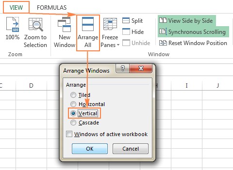
If a vertical arrangement is more suitable for your comparison needs, perhaps for wider datasets, you can easily switch the layout. Click the Arrange All button, also located in the Window group under the View tab. In the Arrange Windows dialog box, select the Vertical option and click OK.

Alt text: Vertically arranged Excel windows showing two different spreadsheets side-by-side, enhancing visual comparison of data in two excel sheets.

This will reorganize your Excel windows, presenting them in a side-by-side vertical format, as illustrated above, which can be particularly effective for comparing columns of data across two sheets.

To enhance the comparison process, especially when you want to scroll through both sheets simultaneously to examine corresponding rows, ensure that Synchronous Scrolling is enabled. This feature is usually activated automatically when you engage the “View Side by Side” mode. You can verify or toggle this setting in the Window group of the View tab, directly beneath the “View Side by Side” button. When activated, scrolling in one window will cause the other to scroll in tandem, keeping corresponding rows aligned for easier comparison.

Alt text: Synchronous scrolling option highlighted in Excel, illustrating its function to simultaneously scroll two excel sheets for parallel data comparison.

For a more detailed guide on utilizing this feature, refer to resources specifically dedicated to viewing Excel workbooks side by side.

1.2. Managing Multiple Excel Windows for Comparison

Extending beyond just two files, Excel allows you to compare data in 2 excel sheets even when you need to view more than two Excel files simultaneously. If you have several workbooks open that you need to compare, clicking the View Side by Side button will initiate the Compare Side by Side dialog box. This dialog will list all currently open workbooks, allowing you to select which files should be displayed alongside the active workbook.

Alt text: Dialog box in Excel showing options to select multiple workbooks for side-by-side comparison, useful when comparing data across several excel sheets.

For a broader overview of all open Excel files at once, the Arrange All button is invaluable. Located in the same Window group on the View tab, clicking “Arrange All” presents several layout options: tiled, horizontal, vertical, or cascade. Choose the arrangement that best suits your comparative task and the number of files you’re working with.

1.3. Comparing Sheets Within the Same Excel Workbook

Often, the need to compare data in 2 Excel sheets arises when the sheets are within the same workbook. To view two sheets from the same workbook side by side, follow these steps:

Open the Excel workbook containing the sheets you wish to compare. Then, go to the View tab and in the Window group, click New Window.
This action opens a second window displaying the same Excel file. Essentially, you now have two independent windows showing the same workbook.
Activate the View Side by Side mode by clicking the corresponding button on the ribbon in either of the windows.
In one of the Excel windows, navigate to and select the first sheet you want to compare. In the other window, select the second sheet.

By following these steps, you can effectively view and compare data in 2 Excel sheets that reside within the same Excel workbook, making visual comparison straightforward and efficient.

2. Formula-Based Comparison: Spotting Value Differences in Excel Sheets

When visual inspection is insufficient or when you need a more structured approach to compare data in 2 Excel sheets, using Excel formulas provides a powerful method to programmatically identify differences in values. This technique is particularly useful for generating a difference report directly within Excel.

To implement a formula-based comparison, you can create a new, empty worksheet that will serve as your difference report. In cell A1 of this new sheet, enter the following formula:

=IF(Sheet1!A1<>Sheet2!A1, "Sheet1:"&Sheet1!A1&" vs Sheet2:"&Sheet2!A1, "")

After entering this formula in cell A1, you need to apply it across the range of cells you wish to compare. You can easily do this by using the fill handle—the small square at the bottom-right corner of the selected cell. Drag the fill handle down and to the right to cover the entire range that corresponds to the data in your original sheets. This action automatically copies the formula, adjusting cell references relative to their new positions.

The use of relative cell references in the formula is crucial. It ensures that as you copy the formula across cells, it dynamically adjusts to compare corresponding cells in Sheet1 and Sheet2. For instance, the formula in cell B1 will compare cell B1 in both Sheet1 and Sheet2, and so on.

The result of this formula is a difference report that highlights cells where the values differ between the two sheets. Where values are identical, the cell in the report remains blank. Where differences exist, the report cell will display a text string indicating the values from both sheets that are different.

Alt text: Excel sheet showing a formula-based comparison report, highlighting value differences between two excel sheets, with discrepancies clearly noted in designated cells.

As illustrated above, the formula effectively identifies cells with differing values and presents these differences in the corresponding cells of the report sheet. It’s important to note, however, that dates in this difference report (like cell C4 in the example) are displayed as serial numbers—Excel’s internal representation of dates. This representation, while accurate, can be less intuitive for quickly analyzing date discrepancies. This method primarily focuses on value comparison and does not extend to comparing formulas or formatting.

3. Conditional Formatting: Visually Highlighting Differences in Excel Sheets

To enhance visual analysis when you compare data in 2 Excel sheets, conditional formatting offers an excellent way to automatically highlight cells that contain different values. This method allows you to apply color coding to discrepancies, making them instantly recognizable.

Here’s how to use conditional formatting to highlight differences:

First, select the worksheet where you want the differences to be highlighted. Choose the entire used range of cells in this sheet. A quick way to do this is by clicking the top-left cell of your data range (usually A1), and then pressing Ctrl + Shift + End to extend the selection to the last used cell.
Navigate to the Home tab on the Excel ribbon. In the Styles group, click on Conditional Formatting, then select New Rule… from the dropdown menu.
In the New Formatting Rule dialog box, choose Use a formula to determine which cells to format. In the formula box, enter the following formula:
```
=A1<>Sheet2!A1
```
Ensure you replace Sheet2 with the actual name of the second sheet you are comparing against.
Click the Format… button to specify how you want the differing cells to be highlighted. Choose your preferred formatting style, such as fill color, font style, or border. Once you have set your formatting preferences, click OK to close the Format Cells dialog, and then click OK again to apply the conditional formatting rule.

As a result, all cells in your selected range that have values different from their corresponding cells in Sheet2 will be highlighted with the color and style you specified.

Alt text: Conditional formatting rule setup in Excel, showing the formula to compare values across two excel sheets and the formatting options to highlight differences.

If you are new to conditional formatting in Excel, detailed guidance can be found in tutorials on Excel conditional formatting based on another cell value.

While formulas and conditional formatting are user-friendly for compare data in 2 excel sheets based on values, they have limitations for comprehensive comparisons:

Value-centric: They only compare cell values and do not account for differences in formulas or cell formatting.
Structural Insensitivity: They cannot detect structural changes like added or deleted rows and columns. If rows or columns are added or removed in one sheet, subsequent row or column comparisons become misaligned, leading to inaccurate difference identification.
Sheet-Level Focus: These methods operate at the sheet level and cannot identify workbook-level structural differences, such as the addition or deletion of entire sheets.

For more in-depth comparisons that address these limitations, consider exploring more advanced Excel features or specialized third-party tools.

4. Compare and Merge Shared Workbooks: Excel’s Built-in Feature for Collaborative Changes

When collaboration is involved and multiple users are working on different copies of the same Excel workbook, Excel’s Compare and Merge Workbooks feature becomes invaluable. This built-in functionality is specifically designed to consolidate changes made by different users into a single primary workbook. It is particularly useful in scenarios where a shared workbook has been distributed, edited by various team members, and needs to be brought back together.

To effectively use the “Compare and Merge” feature, certain preparatory steps are essential:

Share the Workbook: Before distributing the workbook for editing, it must be set up as a shared workbook. To do this, click on the Review tab in Excel, then in the Changes group, click Share Workbook. In the Share Workbook dialog box, ensure the checkbox “Allow changes by more than one user at the same time. This also allows workbook merging” is selected, and click OK. If prompted to save the workbook, allow Excel to do so. Note that enabling the Track Changes feature automatically shares the workbook.
Save Copies with Unique Names: Each person who edits the shared workbook must save their copy with a unique filename. It is crucial that they save it as either an .xls or .xlsx file to ensure compatibility with the merge feature.

Once these preparations are complete, you are ready to use the “Compare and Merge Workbooks” feature to consolidate changes from the various copies.

4.1. Enabling the Compare and Merge Workbooks Command

Although the Compare and Merge Workbooks feature is available in Excel versions from 2010 through Microsoft 365, it is not readily accessible on the Excel ribbon by default. You need to add it to either the Quick Access Toolbar or the ribbon to use it. Here’s how to add it to the Quick Access Toolbar:

Click the dropdown arrow at the end of the Quick Access Toolbar (usually located at the very top left of the Excel window). Select More Commands… from the dropdown menu.
In the Excel Options dialog box, on the left side, choose Quick Access Toolbar. Then, under “Choose commands from,” select All Commands from the dropdown list.
Scroll through the list of commands to find Compare and Merge Workbooks. Select it and click the Add >> button to move it to the right-hand section, which lists the commands currently on your Quick Access Toolbar.
Click OK to close the Excel Options dialog box. The Compare and Merge Workbooks command will now be visible on your Quick Access Toolbar.

Alt text: Excel Options dialog showing how to add the Compare and Merge Workbooks command to the Quick Access Toolbar, making it easily accessible for comparing and merging excel sheets.

4.2. Steps to Compare and Merge Workbooks

With the Compare and Merge Workbooks command now accessible, you can proceed to merge the copies of the shared workbook.

Open the primary version of the shared workbook—this is the workbook into which you want to merge all the changes.
Click the Compare and Merge Workbooks command that you added to the Quick Access Toolbar.
A dialog box will appear, prompting you to select the copies of the shared workbook that you want to merge into the primary workbook. You can select multiple copies by holding down the Shift key while clicking on the filenames. After selecting all relevant copies, click OK.

Alt text: Dialog box prompting selection of workbook copies for merging, step in consolidating changes from multiple users in excel sheets.

Excel will then automatically merge the changes from each selected copy into the primary workbook.

4.3. Reviewing Merged Changes

After merging, it’s crucial to review the changes to understand what modifications were made by different users. Excel provides tools to easily highlight and examine these changes:

Go to the Review tab on the ribbon, and in the Changes group, click Track Changes, then select Highlight Changes… from the dropdown menu.
In the Highlight Changes dialog box, configure the settings to best review the changes:
- In the When dropdown, select All to see all changes made.
- In the Who dropdown, select Everyone to review changes from all users.
- Ensure the Where box is cleared to apply the highlighting across the entire workbook.
- Check the box “Highlight changes on screen”.
- Click OK.

Alt text: Highlight Changes dialog box in Excel, configured to show all changes by everyone on screen, facilitating review of merged changes in excel sheets.

Excel will visually indicate the changes: column letters and row numbers with differences will be highlighted in dark red. At the cell level, edits from different users are marked with different colors. To identify who made a specific change, simply hover your mouse over a highlighted cell, and a tooltip will appear showing the user and the details of the edit.

Important Note: The Compare and Merge Workbooks command is specifically designed for merging copies of a shared workbook. It will not work if you are trying to merge different, unrelated Excel files. Ensure that the workbooks you are attempting to merge are indeed copies of the same originally shared file. If the command appears greyed out, double-check that you are working with a shared workbook and its copies.

5. Third-Party Tools: Advanced Solutions for Excel File Comparison

While Excel offers several built-in methods to compare data in 2 excel sheets, these may not suffice for complex comparison tasks, especially when dealing with large datasets or when you need to compare not just values but also formulas, formatting, and structural elements. For these advanced needs, third-party tools provide more robust and efficient solutions. These tools are specifically designed to offer comprehensive comparison, update, and merging capabilities for Excel sheets and workbooks.

Below is an overview of some leading third-party tools that excel in comparing, updating, and merging Excel files, offering features that go beyond Excel’s native capabilities.

5.1. Synkronizer Excel Compare: A Versatile Tool for Comparison, Merge, and Update

Synkronizer Excel Compare add-in is a powerful tool designed to simplify the process of comparing, merging, and updating Excel files. It is particularly useful for users who need to frequently compare data in 2 excel sheets and require detailed insights into differences and efficient ways to synchronize changes.

Key features of Synkronizer Excel Compare include:

Detailed Difference Identification: Accurately identifies differences between two Excel sheets, including values, formulas, formatting, comments, and named ranges.
Intelligent Merging: Allows for selective merging of differences, preventing unwanted duplications and ensuring data integrity.
Difference Highlighting: Visually highlights all types of differences directly within the sheets, making it easy to spot and understand changes.
Customizable Comparison: Offers options to focus on relevant differences and filter out noise, tailoring the comparison to specific needs.
Comprehensive Reporting: Generates detailed, easy-to-read difference reports that summarize all changes and provide drill-down capabilities.
Sheet and Workbook Updates: Facilitates updating and synchronizing sheets and workbooks based on comparison results.

To illustrate Synkronizer Excel Compare in action, consider a scenario where you are managing event participant data in Excel. You maintain a sheet with participant details, but have two managers who also update their versions of this list. This results in two slightly different Excel files that need to be reconciled.

To use Synkronizer Excel Compare:

Navigate to the Add-ins tab in Excel and click the Synchronizer 11 icon to launch the Synkronizer pane.

Alt text: Synkronizer Excel Compare add-in icon in the Add-ins tab, initiating the tool for excel sheet comparison and merging.
In the Synkronizer pane, select the two Excel workbooks you want to compare.

Alt text: Synkronizer pane showing workbook selection for comparison, enabling users to choose excel sheets for data discrepancy analysis.
Choose the specific sheets within these workbooks to compare. If the workbooks contain sheets with identical names, Synkronizer will automatically match and select them for comparison, as seen with the “Participants” sheets in the example. You can manually adjust sheet selections or configure matching criteria, such as matching by sheet type (all, protected, or hidden).

Alt text: Sheet selection interface in Synkronizer, allowing users to specify which excel sheets within chosen workbooks will be compared for data variations.

Once sheets are selected, Synkronizer can display them side-by-side, similar to Excel’s native “View Side by Side” mode, arranged either vertically or horizontally.
Select a comparison method. Synkronizer offers several options:
- Compare as normal worksheets: The default and most versatile option for general use.
- Compare with link options: Suitable when sheets have the same structure without added or deleted rows/columns, allowing for a “1-on-1” comparison.
- Compare as database: Recommended for sheets structured as databases, enabling more structured comparison.
- Compare selected ranges: Allows you to define specific ranges within sheets for focused comparison.
Optionally, refine the comparison by selecting content types to compare. On the Select tab in the Compare group, you can specify what to include in the comparison:
- Under Content, choose to include comments and names in addition to default comparison of cell values, formulas, and calculated values.
- Under Formats, select cell formats like alignment, fill, font, and border to be compared.
- Use Filters to ignore specific differences, such as case sensitivity, leading/trailing spaces, formula variations that yield the same result, hidden rows/columns, and more.
Finally, click the large red Start button on the ribbon to initiate the comparison process and view the results.

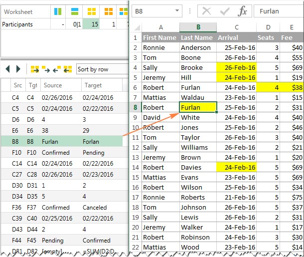
Visualizing and Analyzing Differences with Synkronizer

Synkronizer typically processes and compares sheets rapidly, generating two types of summary reports on the Results tab:

A summary report provides a high-level overview of all difference types found, such as changes in columns, rows, cells, comments, formats, and names.
A detailed difference report is accessible by clicking on a specific difference type in the summary report, providing granular information about each discrepancy.

Alt text: Synkronizer interface displaying a summary report of differences and a detailed report of cell-level discrepancies found between two compared excel sheets.

Clicking on an entry in the detailed report will directly select the corresponding cells in both compared sheets, facilitating immediate review of each difference.

![Direct navigation to differing cells in compared sheets from Synkronizer's difference report.](http://compare.edu.vn/wp-content/uploads/2025/02/view-differences.jpg){width=610 height=515}

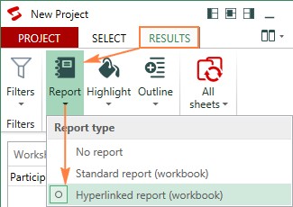
*Alt text: Synkronizer showing navigation to specific differing cells in two excel sheets upon selection in the difference report, aiding in direct comparison and analysis.*

Additionally, Synkronizer can create a difference report in a separate Excel workbook, offering both standard and hyperlinked formats. Hyperlinked reports allow you to click on a difference and jump directly to the corresponding cells in the compared sheets.

![Hyperlinked difference report in a separate Excel workbook generated by Synkronizer.](http://compare.edu.vn/wp-content/uploads/2025/02/hyperlinked-report.jpg){width=325 height=230}

*Alt text: Example of a hyperlinked difference report in Excel created by Synkronizer, enabling quick navigation to discrepancies in compared excel sheets via hyperlinks.*

Comparing All Sheets in Two Workbooks

Synkronizer is capable of comparing all matching sheet pairs within two Excel workbooks simultaneously. The summary report will then present a consolidated view of differences across all compared sheets.

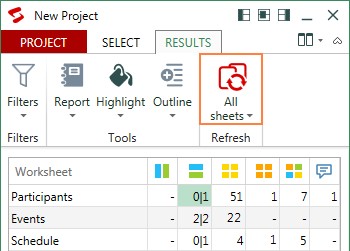![Comparison of all sheets in two workbooks using Synkronizer Excel Compare.](http://compare.edu.vn/wp-content/uploads/2025/02/compare-all-sheets.jpg){width=350 height=251}

*Alt text: Synkronizer's summary report showing comparison results across multiple sheets in two workbooks, providing a comprehensive overview of differences in excel sheets.*

Highlighting Differences Visually

By default, Synkronizer highlights all identified differences directly in the Excel sheets using color codes:

Yellow: Indicates differences in cell values.
Lilac: Denotes differences in cell formats.
Green: Marks inserted rows.

Alt text: Excel sheets with differences highlighted by Synkronizer, using distinct colors to indicate value, format, and structural changes when comparing data in excel sheets.

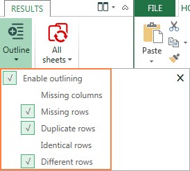
To focus only on specific types of differences, you can use the Outline button on the Results tab to filter and highlight only the differences relevant to your current task.

![Filtering options in Synkronizer to highlight only relevant differences in Excel sheets.](http://compare.edu.vn/wp-content/uploads/2025/02/highlight-relevant-differences.jpg){width=274 height=246}

*Alt text: Synkronizer's Outline options for filtering and highlighting specific types of differences, allowing users to customize the visual comparison of excel sheets.*

Updating and Merging Sheets with Synkronizer

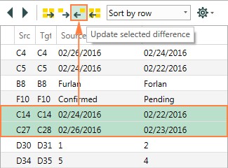
One of Synkronizer’s most valuable features is its merge capability. You can selectively transfer individual cells or entire columns/rows from a source sheet to a target sheet, quickly updating your primary sheet with desired changes.

To update differences, select them in the Synkronizer pane and use one of the four update buttons. The first and last buttons update all differences, while the second and third buttons update only the selected differences, with arrows indicating the direction of data transfer.

![Update and merge sheets using Synkronizer Excel Compare with selective transfer options.](http://compare.edu.vn/wp-content/uploads/2025/02/update-differences.jpg){width=325 height=240}

*Alt text: Synkronizer's update buttons for merging differences between excel sheets, allowing users to selectively transfer and synchronize data changes.*

Synkronizer Excel Compare offers a robust suite of features for anyone needing to efficiently compare data in 2 excel sheets, providing detailed insights, visual aids, and powerful merge capabilities. A trial version of Synkronizer is available for download here.

5.2. Ablebits Compare Sheets for Excel: Intuitive Worksheet Comparison

Ablebits Compare Sheets for Excel, part of their Ultimate Suite, is another excellent tool designed for intuitive worksheet comparison. This add-in focuses on user-friendliness and streamlined workflow, making it easy to compare data in 2 excel sheets effectively.

Key features of Ablebits Compare Sheets include:

Step-by-Step Wizard: Guides users through the comparison process, simplifying configuration and option selection.
Multiple Comparison Algorithms: Offers various algorithms tailored to different data structures, ensuring accurate and relevant comparisons.
Review Differences Mode: Instead of generating a separate report, it displays compared sheets in a “Review Differences” mode, allowing for immediate visual inspection and one-by-one management of differences.
Backup and Safety: Automatically creates backup copies of your original sheets before comparison, ensuring data safety.

To use Ablebits Compare Sheets:

Click the Compare Sheets button located in the Merge group on the Ablebits Data tab in Excel.
The wizard starts by prompting you to select the two worksheets you want to compare. By default, it selects entire sheets, but you can also choose to compare the current table or a specific range by using the respective selection buttons.

Alt text: Ablebits Compare Sheets wizard showing option to select the current table for comparison, enabling users to focus on specific data ranges in excel sheets.

Alt text: Ablebits wizard interface for selecting two excel worksheets to compare, part of a step-by-step process for data comparison in excel sheets.
Choose a comparison algorithm on the next step. Ablebits offers three algorithms:
- No key columns (default): Best for sheet-based documents like invoices or contracts where row order is significant.
- By key columns: Suitable for column-organized sheets with unique identifiers like order numbers or product IDs, allowing for row matching based on keys.
- Cell-by-cell: Ideal for spreadsheets with identical layout and size, such as financial balance sheets or year-over-year reports.
For general purposes, the default “No key columns” option is often effective. Regardless of the algorithm chosen, Ablebits will identify all differences, but the highlighting style (rows or individual cells) may vary.

Additionally, select a match type:
- First match (default): Compares a row in Sheet 1 to the first row in Sheet 2 that has at least one matching cell.
- Best match: Compares a row in Sheet 1 to the row in Sheet 2 that has the maximum number of matching cells, useful for fuzzy matching.
- Full match only: Identifies rows in both sheets that are exactly identical in all cells and marks all other rows as different, useful for finding duplicates or completely unchanged records.
Alt text: Ablebits wizard step for choosing comparison algorithm and match type, offering users flexibility in how excel sheets are compared based on data structure and matching criteria.
Specify which differences to highlight and which to ignore, and choose how differences should be marked. You can configure options to show differences in formatting and ignore hidden rows and columns, tailoring the comparison to your needs.

Alt text: Customization options in Ablebits wizard to select which differences to highlight and ignore, allowing users to refine the comparison output for excel sheets.
Click Compare to start the process. Ablebits will then compare your sheets and display the results in “Review Differences” mode.

Review and Merge Differences in Ablebits

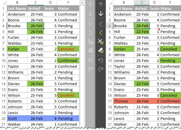
Once processed, the worksheets are presented side-by-side in the Review Differences mode, with the first difference automatically selected.

![Reviewing differences between two worksheets in Ablebits Compare Sheets' Review Differences mode.](http://compare.edu.vn/wp-content/uploads/2025/02/review-worksheets-differences.jpg){width=625 height=449}

*Alt text: Ablebits Review Differences mode showing two excel sheets side-by-side with highlighted differences and a toolbar for managing and reviewing discrepancies.*

In this mode, differences are highlighted with default colors:

Blue rows: Rows present only in Sheet 1 (left side).
Red rows: Rows present only in Sheet 2 (right side).
Green cells: Differing cells within partially matching rows.

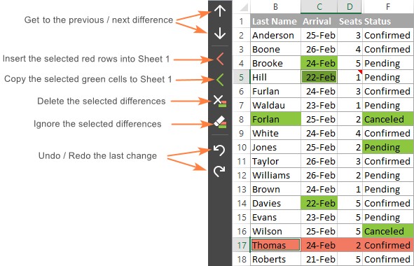
Each worksheet in Review Differences mode has its own vertical toolbar. The toolbar for the inactive sheet is disabled until you select a cell in that sheet. Using these toolbars, you can navigate through each difference one-by-one and decide to either merge or ignore it.

![Review and merge differences using the toolbar in Ablebits Compare Sheets.](http://compare.edu.vn/wp-content/uploads/2025/02/merge-ignore-differences.jpg){width=591 height=380}

*Alt text: Toolbar in Ablebits Review Differences mode with options to navigate, merge, and ignore differences between excel sheets, streamlining the review and reconciliation process.*

After you’ve reviewed all differences, you’ll be prompted to save the workbooks and exit Review Differences mode. If you need to pause review, you can exit and choose to save changes and remove difference marks or restore original workbooks from backups.

Ablebits Compare Sheets offers an intuitive and efficient way to compare data in 2 excel sheets, especially for users who value ease of use and a guided comparison process. A trial version is available for download here.

5.3. xlCompare: Comprehensive Workbook, Sheet, and VBA Project Comparison

xlCompare is a utility designed for comprehensive comparison and merging of Excel files, worksheets, names, and VBA Projects. It excels at identifying additions, deletions, and changes in data, providing tools for quick merging of differences.

Key features of xlCompare include:

Duplicate Record Management: Finds and removes duplicate records between two worksheets.
Record Updating and Merging: Updates existing records in one sheet with values from another and merges updated records between workbooks.
Unique Data Integration: Adds unique rows and columns from one sheet to another.
Data Sorting and Filtering: Sorts data by key columns and filters comparison results to show only differences or identical records.
Visual Highlighting: Highlights comparison results with colors for easy identification of differences.
VBA Project Comparison: Compares VBA projects within Excel workbooks, useful for developers managing code changes.

5.4. Change pro for Excel: Desktop and Mobile Excel Sheet Comparison

Change pro for Excel offers comparison capabilities for Excel sheets on both desktop and mobile devices, with server-based comparison options. It focuses on accuracy and detailed reporting of changes.

Key features of Change pro for Excel include:

Formula and Value Difference Detection: Identifies differences in both formulas and values between two sheets.
Layout Change Recognition: Detects layout changes, including added or deleted rows and columns.
Embedded Object Recognition: Recognizes embedded objects like charts, graphs, and images and reports differences.
Detailed Difference Reports: Creates and prints reports detailing formula, value, and layout differences.
Advanced Filtering and Sorting: Allows filtering, sorting, and searching of difference reports to focus on key changes.
Integration with Outlook and DMS: Compares files directly from Outlook or document management systems.
Multi-Language Support: Supports all languages, including multi-byte character sets.

6. Online Services for Quick Excel File Comparison

For users who need to compare data in 2 excel sheets quickly without installing any software, several online services are available. These services can be particularly useful for one-off comparisons or when working on systems where software installation is restricted. However, consider security implications when uploading sensitive data to online platforms.

Examples of online Excel comparison services include XLComparator and CloudyExcel, among others. These services typically require you to upload two Excel workbooks, and they then perform a comparison and highlight the differences directly in the browser.

Here’s an example of how CloudyExcel works:

Alt text: CloudyExcel online service interface for comparing Excel files, showing file upload options and the comparison initiation button for analyzing data differences in excel sheets.

You simply upload the two Excel workbooks and click a button to “Find Difference.” The service quickly highlights differences in the active sheets using different colors directly in your browser.

Alt text: Excel sheets displayed in CloudyExcel online service with differences highlighted in color, demonstrating quick, browser-based comparison of data in excel sheets.

Online services offer a convenient and fast way to compare data in 2 excel sheets for quick analyses, though they may lack the advanced features and security of desktop software solutions.

Conclusion: Choosing the Right Method to Compare Data in 2 Excel Sheets

Effectively compare data in 2 excel sheets is a fundamental skill for anyone working with Excel. As we’ve explored, there are various methods available, each suited to different needs and levels of complexity.

Visual side-by-side comparison is ideal for quick, manual checks of smaller datasets.
Formula-based comparison and conditional formatting offer structured ways to highlight value differences within Excel sheets, suitable for basic discrepancy identification.
Excel’s Compare and Merge Workbooks feature is tailored for collaborative environments, specifically designed to consolidate changes from shared workbooks.
Third-party tools like Synkronizer Excel Compare, Ablebits Compare Sheets, xlCompare, and Change pro for Excel provide advanced capabilities for comprehensive comparisons, including handling formulas, formatting, structural changes, and offering robust merging and reporting options.
Online services offer immediate, software-free solutions for quick comparisons, balancing convenience with potential security considerations.

Choosing the right method depends on the specific requirements of your task, the complexity of your data, and the level of detail you need in your comparison. For simple tasks, Excel’s built-in features may suffice. However, for more demanding scenarios requiring in-depth analysis, structural comparison, or efficient merging, investing in a third-party tool can significantly enhance your productivity and accuracy.

By mastering these techniques, you can ensure data integrity, streamline your analytical processes, and make more informed decisions based on accurate comparisons of your Excel data. Explore these methods and find the tools that best fit your workflow to optimize how you compare data in 2 excel sheets.

Further Resources for Excel Data Comparison

Other ways to compare and merge data in Excel.