Can You Compare Two Lists in Excel? 5 Effective Methods

Comparing two lists in Excel is crucial for identifying matches, differences, and duplicates. This task is essential for various applications, from managing inventory and customer databases to tracking project tasks and ensuring data accuracy. This guide provides five effective methods to compare two lists in Excel, leveraging formulas, conditional formatting, and built-in tools.

Comparing Lists in Excel: Formulas, Formatting, and More

Excel offers a diverse toolkit for list comparison. Whether you need to highlight duplicates, pinpoint unique entries, or validate data across spreadsheets, mastering these techniques will significantly enhance your data analysis capabilities. Let’s explore five powerful methods:

1. Conditional Formatting for Visual Comparison

Conditional formatting allows you to visually differentiate between matching and non-matching entries.

• Select Data: Select the two lists you want to compare.
• Apply Conditional Formatting: Navigate to Home > Conditional Formatting > Highlight Cells Rules > Duplicate Values.
• Customize: Choose a formatting style to highlight duplicates. To highlight unique values instead, select “Unique” from the dropdown in the Duplicate Values dialog box. This clearly distinguishes entries present in only one list.

.webp)

2. Cell-by-Cell Comparison with the Equal Sign

This method provides a True/False result for each row, indicating whether corresponding cells match.

• Insert Column: Add a new column next to your lists.
• Apply Formula: In the first cell of the new column, enter the formula =A2=B2 (assuming your lists start in A2 and B2).
• Drag Down: Drag the fill handle down to apply the formula to all rows. A “TRUE” indicates a match, while “FALSE” signifies a difference. This allows for a quick scan to identify discrepancies.

.webp)

3. Leveraging the VLOOKUP Formula

VLOOKUP allows you to search for values from one list within another.

• Enter VLOOKUP: In a new column, enter the formula =VLOOKUP(A2,$B$2:$B$9,1,FALSE). Adjust the range $B$2:$B$9 to match your second list.
• Interpret Results: A successful match returns the value from the first list. #N/A indicates the value isn’t found in the second list. This method is particularly helpful for identifying missing items.

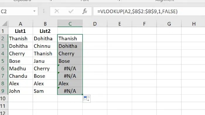Using VLOOKUP to Find Matches Between Lists

4. Identifying Row Differences

This method highlights entire rows where any cell differs between the lists.

• Select Data: Select both lists.
• Go To Special: Press F5 and click “Special.”
• Choose Row Differences: Select “Row differences” and click “OK.” This instantly highlights all rows with discrepancies, enabling quick identification of inconsistencies.

.webp)

5. Using the IF Condition for Clear Results

The IF function provides a more descriptive output, indicating “Matching” or “Not Matching.”

• Apply IF Formula: In a new column, enter =IF(A2=B2,"Matching","Not Matching").
• Drag and Interpret: Drag the formula down. This method provides a clear, text-based result for each row comparison, making it easy to understand at a glance.

.webp)

Conclusion

Comparing two lists in Excel is a fundamental skill for anyone working with data. By utilizing these five methods—conditional formatting, equal sign comparison, VLOOKUP, row differences, and the IF function—you can effectively analyze, validate, and reconcile your data, leading to more accurate insights and informed decisions. Choose the method that best suits your specific needs and data structure for optimal results.