Comparing two columns in Excel to identify differences is a common task for data analysis, list management, and ensuring data integrity. Whether you’re a student, a business professional, or anyone in between, this guide from COMPARE.EDU.VN will provide you with the knowledge and tools necessary to efficiently compare columns and pinpoint discrepancies. Let’s explore the best methods to compare and contrast data in your spreadsheets.
This article explores various methods for comparing two columns in Excel, focusing on formulas, conditional formatting, and third-party tools. By understanding these techniques, you can effectively identify differences and maintain accurate data, making your work with spreadsheets more efficient and reliable. Learn how to enhance data analysis through the effective comparison of Excel data lists.
1. Understanding the Need to Compare Excel Columns
The ability to compare two Excel columns for differences is crucial in various scenarios. These techniques ensure accuracy and facilitate informed decision-making.
1. Data Validation: Ensuring data consistency between two datasets, identifying errors or discrepancies in records.
2. List Management: Identifying unique or duplicate entries when merging or updating lists.
3. Data Cleansing: Spotting inconsistencies in data entries, such as typos or formatting errors.
4. Reconciliation: Matching financial or inventory data to verify accuracy and identify discrepancies.
5. Compliance: Confirming adherence to standards by comparing data against expected values or patterns.
6. Quality Control: Checking if the output data meets specific criteria or expected results by comparing it to a standard.
2. Defining Your Comparison Goals
Before diving into the methods, clarify what you aim to achieve with your comparison.
- Identify Unique Entries: Find values present in one column but not in the other.
- Highlight Differences: Visually mark cells with mismatched data.
- Extract Matching Entries: Copy or flag rows with identical data in both columns.
- Case Sensitivity: Determine if the comparison should distinguish between upper and lower case.
- Partial Matches: Decide if you need to identify partial matches, such as similar text strings.
3. Fundamental Techniques Using Excel Formulas
Excel formulas provide a flexible way to compare columns and highlight differences.
3.1. Comparing Two Columns Row-by-Row for Matches or Differences
This method utilizes the IF function to compare corresponding cells in two columns.
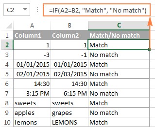
3.1.1. Formula for Exact Matches
The most basic comparison checks for identical values. The following formula compares cells A2 and B2:
=IF(A2=B2, "Match", "No Match")
This formula returns “Match” if the values in A2 and B2 are identical, and “No Match” if they differ.
3.1.2. Formula for Identifying Differences
To specifically highlight differences, use the “<>” operator:
=IF(A2<>B2, "Different", "")
This formula returns “Different” if the values in A2 and B2 are not the same, and an empty string if they match.
3.1.3. Combining Match and Difference Results
A single formula can display both match and difference results:
=IF(A2=B2, "Match", "Different")
Or, alternatively:
=IF(A2<>B2, "Different", "Match")
Here is how this may look in an excel table
| Column A | Column B | Result | Formula |
|---|---|---|---|
| 10 | 10 | Match | =IF(A2=B2, "Match", "Different") |
| 20 | 25 | Different | =IF(A3=B3, "Match", "Different") |
| Apple | Apple | Match | =IF(A4=B4, "Match", "Different") |
| Banana | Orange | Different | =IF(A5=B5, "Match", "Different") |
| 01/01/2024 | 01/01/2024 | Match | =IF(A6=B6, "Match", "Different") |
| 02/15/2024 | 02/20/2024 | Different | =IF(A7=B7, "Match", "Different") |

3.1.4. Handling Case Sensitivity
Standard Excel comparisons are not case-sensitive. To perform a case-sensitive comparison, use the EXACT function:
=IF(EXACT(A2, B2), "Match", "No Match")
This formula returns “Match” only if A2 and B2 are exactly the same, including case.
3.2. Comparing Multiple Columns for Matches
For tables with several columns, you can check for matches across all or any combination of columns.
3.2.1. Finding Matches in All Columns
To find rows where all specified columns have the same values, use the AND function:
=IF(AND(A2=B2, A2=C2), "Full Match", "")
This formula checks if A2 equals both B2 and C2, returning “Full Match” if true.
Alternatively, for a larger number of columns, you can use the COUNTIF function:
=IF(COUNTIF($A2:$E2, $A2)=5, "Full Match", "")
Here, 5 represents the number of columns being compared (A to E).
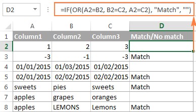
3.2.2. Finding Matches in Any Two Columns
To identify rows where at least two columns match, use the OR function:
=IF(OR(A2=B2, B2=C2, A2=C2), "Match", "")
This formula returns “Match” if any of the specified comparisons are true.
When comparing many columns, the OR statement can become lengthy. A more efficient method is to combine COUNTIF functions:
=IF(COUNTIF(B2:D2,A2)+COUNTIF(C2:D2,B2)+(C2=D2)=0,"Unique","Match")
This formula checks if any two columns in the specified range have the same value, returning “Match” if any match is found.
Here is a demonstration of how to find any matches in multiple columns:
| Column A | Column B | Column C | Result | Formula |
|—|—|—|—|
| 10 | 10 | 15 | Match | =IF(OR(A2=B2, B2=C2, A2=C2), "Match", "") |
| 20 | 25 | 25 | Match | =IF(OR(A3=B3, B3=C3, A3=C3), "Match", "") |
| Apple | Orange | Banana | Unique | =IF(OR(A4=B4, B4=C4, A4=C4), "Match", "") |
| Grape | Grape | Grape | Match | =IF(OR(A5=B5, B5=C5, A5=C5), "Match", "") |
3.3. Comparing Two Columns for Matches and Differences Across Entire Lists
Sometimes you need to compare two columns to find values in one column that do not exist in the other.
3.3.1. Identifying Unique Values in Column A
To find values in column A that are not present in column B, use the COUNTIF function:
=IF(COUNTIF($B:$B, $A2)=0, "No match in B", "")
This formula checks the entire column B for each value in column A. If no match is found, it returns “No match in B”.
3.3.2. Alternative Formula Using ISERROR and MATCH
An alternative approach uses the ISERROR and MATCH functions:
=IF(ISERROR(MATCH($A2,$B$2:$B$10,0)),"No match in B","")
This formula checks if the value in A2 is found in the range B2:B10. If not found, it returns “No match in B”.
3.3.3. Formula for Identifying Matches and Differences
To display both matches and differences, combine the COUNTIF function with conditional text:
=IF(COUNTIF($B:$B, $A2)=0, "No match in B", "Match in B")
This formula returns “No match in B” if the value in A2 is not found in column B, and “Match in B” if it is found.
3.3.4. Specifying a Range Instead of an Entire Column
For larger datasets, specifying a range instead of the entire column can improve performance:
=IF(COUNTIF($B$2:$B$100, $A2)=0, "No match in B", "Match in B")
This limits the search to rows 2 through 100 in column B.
4. Advanced Techniques: VLOOKUP, INDEX MATCH, and XLOOKUP
These functions are essential for extracting matching data and performing more complex comparisons.
4.1. Using VLOOKUP to Pull Matching Data
The VLOOKUP function is used to find a value in one column and return a corresponding value from another column.
=VLOOKUP(D2, $A$2:$B$6, 2, FALSE)
This formula searches for the value in D2 within the range A2:A6 and returns the corresponding value from the second column (B) in the range.
4.2. Using INDEX MATCH for More Flexible Lookups
The INDEX MATCH combination is more versatile than VLOOKUP because it can look up values to the left.
=INDEX($B$2:$B$6, MATCH($D2, $A$2:$A$6, 0))
This formula finds the position of the value in D2 within the range A2:A6 using MATCH, and then returns the value from the corresponding position in the range B2:B6 using INDEX.
4.3. Using XLOOKUP for Enhanced Lookups (Excel 365 and Later)
XLOOKUP is a newer function that combines the strengths of VLOOKUP and INDEX MATCH with additional features.
=XLOOKUP(D2, $A$2:$A$6, $B$2:$B$6)
This formula searches for the value in D2 within the range A2:A6 and returns the corresponding value from the range B2:B6. XLOOKUP is more intuitive and can handle errors more gracefully than VLOOKUP.
Example of a VLOOKUP formula
| Product ID | Sales Figure |
|---|---|
| 101 | 500 |
| 102 | 750 |
| 103 | 600 |
| 104 | 800 |
| 105 | 700 |
| Product ID (Lookup) | Sales Figure (VLOOKUP) | VLOOKUP Formula |
|---|---|---|
| 103 | 600 | =VLOOKUP(D2, $A$2:$B$6, 2, FALSE) |
| 106 | #N/A | =VLOOKUP(D3, $A$2:$B$6, 2, FALSE) |
| 101 | 500 | =VLOOKUP(D4, $A$2:$B$6, 2, FALSE) |
This is how you can compare two columns using the VLOOKUP Formula.
5. Visual Comparison Using Conditional Formatting
Conditional formatting is an essential feature of Microsoft Excel that allows users to automatically apply formatting (such as colors, icons, and data bars) to cells based on their values or the results of formulas. It is incredibly useful for visually analyzing data, identifying trends, and highlighting important information.
5.1. Highlighting Matches and Differences in Each Row
Conditional formatting can visually highlight matching or differing entries in two columns.
5.1.1. Highlighting Identical Entries
To highlight cells in column A that match entries in column B, follow these steps:
- Select the cells in column A.
- Go to Conditional Formatting > New Rule > Use a formula to determine which cells to format.
- Enter the formula:
=$B2=$A2 - Choose a formatting style (e.g., fill color) and click OK.
This highlights cells in column A that have identical entries in the corresponding row of column B.
5.1.2. Highlighting Differences
To highlight cells with different entries, use the formula:
=$B2<>$A2
This highlights cells in column A that do not match the entries in the corresponding row of column B.
5.2. Highlighting Unique Entries in Each List
Conditional formatting can also highlight items that appear in only one of the two lists.
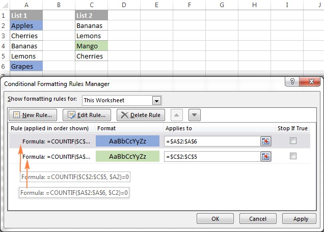
5.2.1. Highlighting Unique Values in List 1 (Column A)
Use the following formula:
=COUNTIF($C$2:$C$5, $A2)=0
This highlights values in column A that do not appear in the range C2:C5 (List 2).
5.2.2. Highlighting Unique Values in List 2 (Column C)
Use the following formula:
=COUNTIF($A$2:$A$6, $C2)=0
This highlights values in column C that do not appear in the range A2:A6 (List 1).
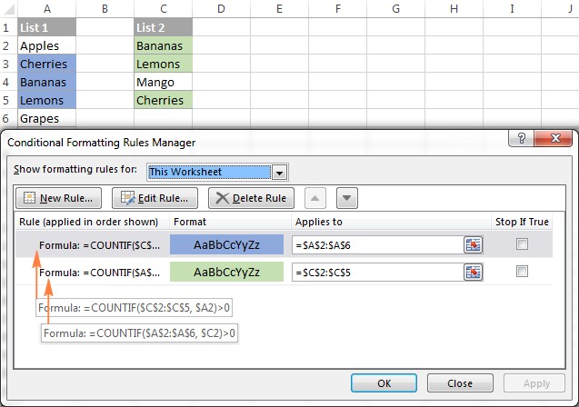
5.3. Highlighting Matches (Duplicates) Between Two Columns
To highlight items that appear in both columns, adjust the COUNTIF formulas to look for counts greater than zero.
5.3.1. Highlighting Matches in List 1 (Column A)
Use the formula:
=COUNTIF($C$2:$C$5, $A2)>0
This highlights values in column A that also appear in the range C2:C5.
5.3.2. Highlighting Matches in List 2 (Column C)
Use the formula:
=COUNTIF($A$2:$A$6, $C2)>0
This highlights values in column C that also appear in the range A2:A6.
6. Comparing Rows in Multiple Columns
You can compare rows across multiple columns to identify matches or differences in entire records.
6.1. Highlighting Rows with Identical Values in All Columns
To highlight rows where all values in the specified columns are the same, use a conditional formatting rule based on the AND or COUNTIF function.
6.1.1. Using the AND Function
=AND($A2=$B2, $A2=$C2)
This formula highlights rows where A2, B2, and C2 are all equal.
6.1.2. Using the COUNTIF Function
=COUNTIF($A2:$C2, $A2)=3
This formula highlights rows where the count of cells equal to A2 in the range A2:C2 is 3 (the number of columns being compared).
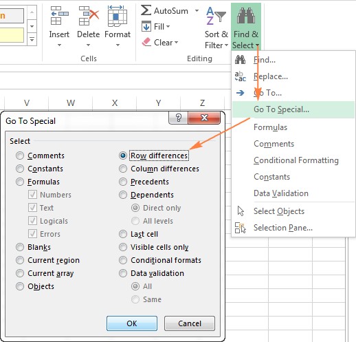
6.2. Highlighting Rows with Differences Using “Go To Special”
Excel’s “Go To Special” feature offers a quick way to highlight cells with different values in each row.
- Select the range of cells you want to compare (e.g., A2:C8). The top-left cell is the active cell.
- Go to Home > Editing > Find & Select > Go To Special.
- Select Row differences and click OK.
- The cells with values different from the active cell in each row will be selected.
- Apply a fill color to highlight the selected cells.
This approach is particularly useful for visually identifying discrepancies in large datasets.
7. Comparing Two Individual Cells
Comparing two individual cells is a simple case of row-by-row comparison without the need to copy formulas.
7.1. Formula for Matches
=IF(A1=C1, "Match", "")
7.2. Formula for Differences
=IF(A1<>C1, "Difference", "")
These formulas provide immediate feedback on whether the values in the two cells are the same or different.
8. Formula-Free Comparison with Third-Party Tools
While Excel formulas and conditional formatting are powerful, third-party tools can offer more intuitive and advanced comparison options.
8.1. Introducing Ablebits Compare Two Tables
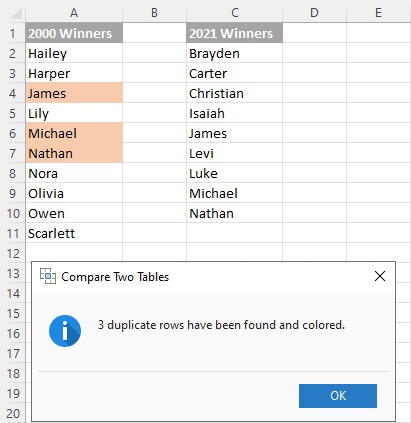
The Ablebits Compare Two Tables add-in is designed to compare two tables or lists, identify matches and differences, and highlight them in various ways. This tool simplifies the comparison process and provides additional features not available in standard Excel.
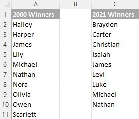
8.2. Steps to Compare Lists Using Ablebits
- Click the Compare Tables button on the Ablebits Data tab.
- Select the first column/list (Table 1) and click Next.
- Select the second column/list (Table 2) and click Next.
- Choose whether to search for Duplicate values (matches) or Unique values (differences) and click Next.
- Select the columns for comparison and click Next.
- Choose how to handle the found items:
- Highlight with color: Shades matches or differences in the selected color.
- Identify in the Status column: Inserts a Status column with “Duplicate” or “Unique” labels.
- Click Finish to apply the comparison.
8.3. Highlighting and Identifying Matches
The Ablebits add-in can highlight matches or differences and add a status column to indicate whether each entry is a duplicate or unique.
9. Best Practices for Comparing Excel Columns
To ensure accurate and efficient comparisons, follow these best practices:
- Clean Your Data: Remove any inconsistencies such as extra spaces or incorrect formatting.
- Sort Your Data: Sorting data before comparison can make identifying patterns and differences easier.
- Use Consistent Formulas: Apply the same formula consistently across all rows to avoid errors.
- Test Your Formulas: Verify that your formulas are working correctly by testing them on a small subset of data.
- Specify Ranges: Whenever possible, specify ranges instead of entire columns to improve performance.
- Document Your Steps: Keep a record of the comparison steps and formulas used for future reference and auditing.
- Regularly Update Your Skills: Stay informed about new Excel features and techniques to improve your comparison capabilities.
10. FAQ: Comparing Two Excel Columns for Differences
1. How do I compare two columns in Excel for differences?
Use the IF function with the “<>” operator to identify different values in corresponding rows.
2. How can I highlight differences between two columns in Excel?
Use conditional formatting with a formula like “=$A2<>$B2” to highlight cells with different values.
3. How do I find unique values in two columns in Excel?
Use the COUNTIF function in conditional formatting to highlight values that appear only in one column.
4. How can I compare two columns in Excel for matches?
Use the IF function with the “=” operator or conditional formatting to highlight matching values.
5. What is the best way to compare two large columns in Excel?
Use formulas with specified ranges instead of entire columns, or consider using third-party add-ins like Ablebits Compare Two Tables.
6. How do I perform a case-sensitive comparison in Excel?
Use the EXACT function within an IF formula to compare text values case-sensitively.
7. Can I compare multiple columns for differences at once?
Yes, use the “Go To Special” feature to highlight row differences across multiple selected columns.
8. How do I extract matching values from two columns in Excel?
Use the VLOOKUP, INDEX MATCH, or XLOOKUP functions to retrieve matching values from one column based on another.
9. What are the alternatives to using formulas for comparing columns?
Third-party add-ins like Ablebits Compare Two Tables offer more intuitive interfaces and additional features for comparing columns.
10. How do I ensure the accuracy of my column comparisons in Excel?
Clean your data, use consistent formulas, test your formulas, and document your steps to ensure accurate results.
11. Conclusion: Making Informed Decisions with Accurate Data
Comparing two columns in Excel for differences is a fundamental skill that enhances data analysis and decision-making. Whether you use basic formulas, advanced functions, conditional formatting, or third-party tools, the methods discussed in this guide from COMPARE.EDU.VN will help you efficiently identify discrepancies, maintain data integrity, and make informed decisions. With these techniques, you can ensure the accuracy and reliability of your spreadsheets, leading to more effective outcomes in your personal and professional endeavors.
Ready to take your data comparison skills to the next level? Visit COMPARE.EDU.VN for more in-depth guides and resources that will empower you to make the best decisions based on accurate and reliable data. Contact us at 333 Comparison Plaza, Choice City, CA 90210, United States or reach out via WhatsApp at +1 (626) 555-9090. Visit our website at compare.edu.vn to explore more!