Can You Compare Posterior Mode and Median Dynare?

COMPARE.EDU.VN explores the nuanced relationship between posterior mode and median within the Dynare framework, providing clarity for econometric modelers. Navigating the complexities of Bayesian estimation can be challenging, but this comprehensive guide offers a clear comparison, empowering you to make informed decisions about your model specification and estimation techniques. Explore alternative optimization routines and parameter initialization for superior outcomes, increasing your understanding of econometric tools and techniques.

1. Understanding Posterior Mode and Median in Bayesian Econometrics

In Bayesian econometrics, the posterior distribution represents our updated belief about model parameters after observing the data. It combines the prior belief with the information from the likelihood function. The posterior mode and median are two key measures of central tendency for this distribution, but they capture different aspects and can lead to different inferences.

1.1. Posterior Mode: Finding the Peak

The posterior mode is the value of the parameter that maximizes the posterior density function. In simpler terms, it’s the “most likely” value of the parameter given the data and the prior. It’s often found using optimization algorithms like those implemented in Dynare.

Characteristics of the Posterior Mode:

Point Estimate: The posterior mode provides a single point estimate for each parameter.
Optimization-Based: It’s determined by finding the maximum of the posterior density.
Sensitivity to Prior: The mode can be sensitive to the choice of prior, especially with weak data.
May Not Be Representative: In skewed or multi-modal distributions, the mode may not be a representative value of the distribution’s center.

1.2. Posterior Median: The Middle Ground

The posterior median is the value that divides the posterior distribution into two equal halves. Half of the probability mass lies below the median, and half lies above. It is typically computed using Markov Chain Monte Carlo (MCMC) methods.

Characteristics of the Posterior Median:

Robust to Outliers: The median is less sensitive to extreme values (outliers) than the mode.
Represents Central Tendency: It provides a more robust measure of the distribution’s central tendency, especially in skewed distributions.
Computational Cost: Calculating the median requires MCMC simulations, which can be computationally intensive.
Less Sensitive to Prior: Compared to the mode, the median is generally less affected by the prior specification, especially with informative data.

1.3. Visualizing the Difference

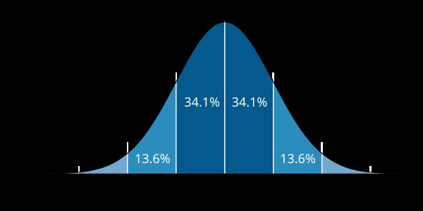
Imagine a probability distribution shaped like a hill. The posterior mode is the highest point of the hill, while the posterior median is the point that splits the area under the curve into two equal halves. In a perfectly symmetrical hill, the mode and median would coincide. However, if the hill is skewed (leaning to one side), the mode and median will be different.

2. Dynare and Bayesian Estimation: A Powerful Combination

Dynare is a widely used software package for solving and estimating dynamic stochastic general equilibrium (DSGE) models. It provides a suite of tools for Bayesian estimation, including algorithms for finding the posterior mode and MCMC methods for characterizing the entire posterior distribution.

2.1. Finding the Posterior Mode in Dynare

Dynare uses optimization routines (e.g., fmincon, csminwel) to find the posterior mode. This involves maximizing the posterior kernel, which is proportional to the posterior density. The estimation command in Dynare handles this process.

Steps to Find the Posterior Mode in Dynare:

Specify the Model: Define the DSGE model in a .mod file.
Declare Parameters and Priors: Specify the parameters to be estimated and their prior distributions.
Run the Estimation Command: Use the estimation command with options to control the optimization algorithm.

Example:

var y, c, k, a, r;
varexo e;

parameters beta, rho, alpha, delta, sigma;

beta = 0.99;
rho  = 0.95;
alpha = 0.36;
delta = 0.025;
sigma = 1.5;

model;
c + k = y;
y = a*k(-1)^alpha;
c^(-sigma) = beta*c(+1)^(-sigma)*(1+r(+1)-delta);
r = alpha*a*k(-1)^(alpha-1);
a = rho*a(-1) + e;
end;

initval;
k = (alpha*beta*a)^(1/(1-alpha));
y = a*k^alpha;
c = y-delta*k;
r = alpha*a*k^(alpha-1);
a = 1;
e = 0;
end;

varexo e;
stderr e 0.01;

estimated_params;
  beta, beta_pdf, 0.99, 0.02;
  rho, beta_pdf, 0.95, 0.05;
  alpha, beta_pdf, 0.36, 0.02;
  delta, normal_pdf, 0.025, 0.005;
  sigma, normal_pdf, 1.5, 0.25;
stderr e, inv_gamma_pdf, 0.01, 2;
end;

estimation(datafile=data, mode_compute=6, mh_replic=2000, mh_nblocks=2, mh_jscale=0.2);

Common Issues When Finding the Posterior Mode:

Non-Positive Definite Hessian: This error indicates that the optimization algorithm has not converged to a true maximum. Possible solutions include:
- Changing the optimization algorithm (mode_compute).
- Providing better starting values for the parameters (estimated_params_init).
- Checking for model misspecification.
Error Using Chol: This error suggests that the covariance matrix of the parameters is not positive definite, often due to identification problems.

2.2. Computing the Posterior Median in Dynare

Dynare uses MCMC methods, specifically the Metropolis-Hastings algorithm, to simulate draws from the posterior distribution. The posterior median is then calculated from these draws.

Steps to Compute the Posterior Median in Dynare:

Find the Posterior Mode: As a starting point for the MCMC sampler.
Run the Estimation Command with MCMC Options: Use the estimation command with options like mh_replic, mh_nblocks, and mh_jscale to control the MCMC simulation.

Example (Continued from Above):

estimation(datafile=data, mode_compute=6, mh_replic=50000, mh_nblocks=2, mh_jscale=0.2);

Interpreting the Results:

After running the estimation, Dynare provides summary statistics for the posterior distribution, including the median, mean, standard deviation, and credible intervals.

2.3. Dynare’s Importance in Econometric Comparisons

Dynare streamlines the comparison of posterior mode and median in several ways:

Automated Estimation: Dynare automates the complex processes of mode-finding and MCMC simulation.
Diagnostic Tools: It offers diagnostic plots and statistics to assess convergence and the quality of the MCMC draws.
Flexibility: Dynare allows users to customize the estimation procedure, including the choice of optimization algorithms, prior distributions, and MCMC settings.
Model Evaluation: Dynare simplifies model evaluation through posterior analysis, enabling users to compare different models and assess their fit to the data.
Open Source: Being open source, Dynare is transparent and customizable, making it a reliable tool for advanced econometric analysis.

3. Comparing Posterior Mode and Median: A Detailed Analysis

When should you use the posterior mode, and when is the posterior median more appropriate? The answer depends on the characteristics of the posterior distribution and the goals of your analysis.

3.1. Scenarios Where the Posterior Mode is Useful

Model Comparison: The posterior mode is often used in model comparison through the modified information criteria. The mode provides a quick and easy way to evaluate the likelihood of the data under different models.
Initialization for MCMC: The posterior mode serves as a good starting point for MCMC simulations. Starting the MCMC chain near the mode can improve convergence and efficiency.
Approximation of the Posterior: When computational resources are limited, the posterior mode can provide a reasonable approximation of the posterior distribution.

3.2. Scenarios Where the Posterior Median is Preferred

Skewed Distributions: When the posterior distribution is skewed, the median provides a more representative measure of central tendency than the mode.
Robustness to Outliers: The median is less sensitive to extreme values, making it a more robust estimator in the presence of outliers or influential data points.
Decision-Making: In decision-making contexts, the median may be more appropriate when the cost function is asymmetric. For example, if overestimating a parameter has a different cost than underestimating it, the median minimizes the expected loss.

3.3. Practical Considerations

Computational Cost: Finding the posterior mode is generally faster than computing the posterior median using MCMC. This can be a significant factor when dealing with large models or datasets.
Convergence: MCMC simulations require careful monitoring of convergence. It’s essential to ensure that the MCMC chain has explored the entire posterior distribution before calculating the median.
Prior Sensitivity: Both the mode and median can be affected by the choice of prior. It’s important to perform sensitivity analysis to assess the impact of different prior specifications on the results.

3.4. Comparative Analysis: Posterior Mode vs. Posterior Median

Feature	Posterior Mode	Posterior Median
Definition	Value that maximizes the posterior density	Value that divides the posterior distribution in half
Computation	Optimization algorithms (e.g., `fmincon`)	MCMC methods (e.g., Metropolis-Hastings)
Sensitivity to Prior	Higher sensitivity	Lower sensitivity
Robustness to Outliers	Lower robustness	Higher robustness
Computational Cost	Lower cost	Higher cost
Use Cases	Model comparison, initialization for MCMC	Skewed distributions, robust estimation

Posterior Mode vs Median

Alt Text: Illustration comparing the position of the mean (average), median (middle value), and mode (most frequent value) in a skewed distribution, highlighting how the mode represents the peak while the median divides the area equally.

4. Addressing Common Issues and Troubleshooting

When working with Dynare and Bayesian estimation, you may encounter various issues. Here’s a guide to troubleshooting some common problems.

4.1. Dealing with Non-Positive Definite Hessian

A non-positive definite Hessian matrix at the posterior mode indicates that the optimization algorithm has not converged to a true maximum. This can happen due to several reasons:

Model Misspecification: The model may not be a good fit for the data.
Identification Problems: The parameters may not be uniquely identified by the data.
Poor Starting Values: The optimization algorithm may have started from a point far from the true mode.
Algorithm Choice: The default optimization algorithm may not be suitable for the problem.

Solutions:

Check Model Specification: Review the model equations and ensure they are correctly specified. Look for potential sources of misspecification, such as omitted variables or incorrect functional forms.
Address Identification Issues: Ensure that each parameter is uniquely identified by the data. This may involve adding more data, imposing additional restrictions, or reparameterizing the model.
Provide Better Starting Values: Use the estimated_params_init block in Dynare to provide better starting values for the parameters. You can try using values from previous estimations or from theoretical considerations.
Change Optimization Algorithm: Experiment with different optimization algorithms using the mode_compute option in Dynare. For example, try mode_compute=6 (csminwel) or mode_compute=9 (a more robust algorithm).
Increase Optimization Iterations: Increase the maximum number of iterations for the optimization algorithm using the maxfun option.

4.2. Resolving “Error Using Chol”

The “Error using chol” indicates that the covariance matrix of the parameters is not positive definite. This often occurs when the model is not properly identified, leading to a singular covariance matrix.

Solutions:

Address Identification Issues: As with the non-positive definite Hessian, ensure that each parameter is uniquely identified by the data.
Check for Collinearity: Look for highly correlated parameters, which can cause the covariance matrix to be singular.
Regularization: Add a small amount of regularization to the covariance matrix to make it positive definite. This can be done by adding a small positive constant to the diagonal elements of the matrix. However, use this approach with caution, as it can bias the results.
Prior Specification: Review the prior distributions. Non-informative priors might lead to issues. Try using more informative priors to guide the estimation process.

4.3. Improving MCMC Convergence

MCMC simulations can be slow to converge, especially for complex models with many parameters. Here are some tips to improve convergence:

Start from the Posterior Mode: As mentioned earlier, starting the MCMC chain near the posterior mode can significantly improve convergence.
Tune the MCMC Sampler: Adjust the MCMC settings, such as the number of blocks (mh_nblocks) and the scaling factor (mh_jscale), to optimize the sampler’s performance.
Increase the Number of Replications: Increase the number of MCMC replications (mh_replic) to obtain more accurate estimates of the posterior distribution.
Monitor Convergence Diagnostics: Use Dynare’s diagnostic plots and statistics to monitor convergence. Look for signs of non-convergence, such as trends in the MCMC chain or high autocorrelation.
Thin the MCMC Chain: If the MCMC chain is highly autocorrelated, thin the chain by saving only every nth draw. This can reduce the storage requirements and improve the accuracy of the posterior estimates.

4.4. Handling Prior Sensitivity

The choice of prior can have a significant impact on the posterior distribution, especially with limited data. It’s important to assess the sensitivity of the results to different prior specifications.

Strategies for Addressing Prior Sensitivity:

Experiment with Different Priors: Try using different prior distributions for the parameters. For example, compare the results obtained with normal priors, uniform priors, and beta priors.
Use Informative Priors: Incorporate prior knowledge into the prior distributions. This can help to guide the estimation process and reduce the impact of the data.
Perform Robustness Checks: Conduct robustness checks to assess the sensitivity of the results to different prior specifications. If the results are highly sensitive to the choice of prior, consider reporting results for multiple priors.

Alt Text: Graph illustrating prior sensitivity analysis by showing how different prior distributions affect the resulting posterior distributions for a parameter, demonstrating the impact of prior choices on estimation outcomes.

5. Advanced Techniques and Considerations

Beyond the basic comparison of posterior mode and median, several advanced techniques and considerations can enhance your Bayesian estimation in Dynare.

5.1. Model Identification

Model identification is crucial for reliable Bayesian estimation. A model is identified if the parameters can be uniquely estimated from the data. Unidentified models can lead to non-positive definite Hessian matrices, “Error using chol,” and poor MCMC convergence.

Techniques for Assessing Model Identification:

Rank Condition: Check the rank condition for local identification. This involves verifying that the Jacobian matrix of the model’s equilibrium conditions has full rank.
Information Matrix: Examine the information matrix to assess the degree of identification. A singular information matrix indicates that the model is not identified.
Posterior плотность: Examine the posterior density to assess the shape and spread of the distribution. A flat or highly dispersed posterior density may indicate identification problems.

5.2. Prior Choice and Elicitation

The choice of prior can significantly impact the posterior distribution. It’s essential to carefully consider the prior distributions and, if possible, elicit priors from experts.

Strategies for Prior Choice:

Non-Informative Priors: Use non-informative priors when little is known about the parameters. However, be aware that non-informative priors can sometimes lead to improper posterior distributions.
Informative Priors: Incorporate prior knowledge into the prior distributions. This can help to guide the estimation process and improve the accuracy of the results.
Hierarchical Priors: Use hierarchical priors to model the uncertainty about the prior distributions themselves. This can be particularly useful when dealing with multiple related parameters.

5.3. MCMC Diagnostics and Convergence Assessment

MCMC simulations require careful monitoring of convergence. Several diagnostic tools can help to assess whether the MCMC chain has converged to the posterior distribution.

Common MCMC Diagnostics:

Trace Plots: Examine the trace plots of the MCMC chain to look for trends, cycles, or other signs of non-convergence.
Autocorrelation Plots: Examine the autocorrelation plots to assess the degree of autocorrelation in the MCMC chain. High autocorrelation can indicate slow convergence.
Gelman-Rubin Statistic: Compute the Gelman-Rubin statistic to compare the within-chain and between-chain variance. Values close to 1 indicate convergence.
Effective Sample Size: Calculate the effective sample size to estimate the number of independent draws from the posterior distribution.

5.4. Bayesian Model Comparison

Bayesian model comparison involves comparing the posterior probabilities of different models. This can be done using Bayes factors or posterior model probabilities.

Methods for Bayesian Model Comparison:

Bayes Factors: Compute the Bayes factor for each pair of models. The Bayes factor is the ratio of the marginal likelihoods of the two models.
Posterior Model Probabilities: Compute the posterior model probabilities by normalizing the marginal likelihoods. The posterior model probability represents the probability that a given model is the true model, given the data.
Deviance Information Criterion (DIC): The DIC is a measure of model fit that penalizes model complexity. Models with lower DIC values are preferred.
Widely Applicable Information Criterion (WAIC): WAIC is a more general measure of model fit that can be used for both regular and singular models.

6. Practical Examples and Case Studies

To illustrate the comparison of posterior mode and median, let’s consider a couple of practical examples.

6.1. Example 1: Estimating a Simple Macroeconomic Model

Consider a simple New Keynesian model with sticky prices and monetary policy rule. The model includes parameters such as the elasticity of substitution, the degree of price stickiness, and the central bank’s response to inflation.

Scenario:

The posterior distribution for the elasticity of substitution is slightly skewed due to the presence of some influential data points.
The posterior distribution for the central bank’s response to inflation is approximately symmetric.

Results:

For the elasticity of substitution, the posterior median provides a more robust estimate of the central tendency than the posterior mode.
For the central bank’s response to inflation, the posterior mode and median are very similar, indicating that either measure can be used.

6.2. Example 2: Estimating a DSGE Model with Financial Frictions

Consider a DSGE model with financial frictions, such as borrowing constraints and financial intermediaries. The model includes parameters such as the degree of borrowing constraints, the risk aversion of households, and the capital adequacy ratio of banks.

Scenario:

The posterior distribution for the degree of borrowing constraints is highly skewed due to the presence of a few extreme events, such as financial crises.
The posterior distribution for the risk aversion of households is approximately symmetric.

Results:

For the degree of borrowing constraints, the posterior median is a more appropriate measure of central tendency than the posterior mode. The median is less sensitive to the extreme events and provides a more stable estimate.
For the risk aversion of households, the posterior mode and median are similar, indicating that either measure can be used. However, it’s important to check the robustness of the results to different prior specifications.

7. Future Trends and Developments

Bayesian estimation in Dynare is an active area of research, and several exciting developments are on the horizon.

7.1. Improved MCMC Algorithms

Researchers are continuously developing new and improved MCMC algorithms that can converge faster and explore the posterior distribution more efficiently. Examples include Hamiltonian Monte Carlo (HMC) and Sequential Monte Carlo (SMC).

7.2. Automated Convergence Diagnostics

Automated convergence diagnostics can help to streamline the MCMC process and reduce the need for manual monitoring. These diagnostics use statistical tests and machine learning techniques to assess convergence automatically.

7.3. More Flexible Prior Specifications

More flexible prior specifications can allow researchers to incorporate more complex prior beliefs into the estimation process. Examples include non-parametric priors and mixture priors.

7.4. Integration with Machine Learning Techniques

Integrating machine learning techniques with Bayesian estimation can help to improve model identification, prior elicitation, and convergence diagnostics. For example, machine learning algorithms can be used to estimate the prior distribution from historical data or to detect non-convergence in MCMC chains.

8. Conclusion: Making Informed Choices

Choosing between the posterior mode and median in Dynare depends on the specific characteristics of your model, data, and research question. While the mode offers computational efficiency and is useful for model comparison, the median provides a more robust measure of central tendency, especially in skewed distributions. By understanding the strengths and weaknesses of each measure, you can make informed decisions and obtain more reliable results. Remember to carefully assess model identification, prior sensitivity, and MCMC convergence to ensure the validity of your findings. Visit COMPARE.EDU.VN at 333 Comparison Plaza, Choice City, CA 90210, United States, or contact us on Whatsapp at +1 (626) 555-9090 for further assistance in comparing econometric methods.

9. Call to Action

Are you struggling to compare different econometric models and make informed decisions about your research? Do you need help understanding the nuances of Bayesian estimation in Dynare?

Visit COMPARE.EDU.VN today to find detailed comparisons of different econometric techniques, including the posterior mode and median. Our comprehensive resources will help you:

Understand the strengths and weaknesses of different estimation methods
Choose the most appropriate method for your research question
Troubleshoot common issues and improve the reliability of your results

Don’t waste time and effort on trial and error. Let COMPARE.EDU.VN guide you to the best decisions for your econometric analysis. Contact us at 333 Comparison Plaza, Choice City, CA 90210, United States or on Whatsapp at +1 (626) 555-9090, or visit our website COMPARE.EDU.VN.

10. Frequently Asked Questions (FAQ)

10.1. What is the posterior distribution?

The posterior distribution represents the updated belief about model parameters after observing the data. It combines the prior belief with the information from the likelihood function.

10.2. What is the difference between the posterior mode and median?

The posterior mode is the value of the parameter that maximizes the posterior density function, while the posterior median is the value that divides the posterior distribution into two equal halves.

10.3. When should I use the posterior mode?

The posterior mode is useful for model comparison and as a starting point for MCMC simulations.

10.4. When should I use the posterior median?

The posterior median is preferred when the posterior distribution is skewed or when robustness to outliers is important.

10.5. How do I find the posterior mode in Dynare?

Use the estimation command in Dynare with options to control the optimization algorithm.

10.6. How do I compute the posterior median in Dynare?

Use the estimation command with MCMC options, such as mh_replic, mh_nblocks, and mh_jscale.

10.7. What is a non-positive definite Hessian?

A non-positive definite Hessian matrix at the posterior mode indicates that the optimization algorithm has not converged to a true maximum.

10.8. How can I improve MCMC convergence?

Start from the posterior mode, tune the MCMC sampler, increase the number of replications, and monitor convergence diagnostics.

10.9. How can I assess prior sensitivity?

Experiment with different prior distributions and perform robustness checks.

10.10. Where can I find more information about Bayesian estimation in Dynare?

Visit COMPARE.EDU.VN or contact us on Whatsapp at +1 (626) 555-9090 for further assistance and detailed comparisons.

This comprehensive guide, brought to you by compare.edu.vn, provides a thorough comparison of the posterior mode and median in Dynare, equipping you with the knowledge and tools to make informed decisions in your econometric modeling.