Can You Compare Posterior Mode And Median?

At COMPARE.EDU.VN, understanding the nuances between the posterior mode and median is crucial for robust Bayesian statistical analysis. This article provides a comprehensive exploration, optimized for search engines, covering their definitions, applications, and advantages. Dive into the world of statistical measures with us, enhancing your data interpretation skills.

1. Introduction to Posterior Mode and Median

In Bayesian inference, the posterior distribution is a central concept that combines prior beliefs with evidence from observed data. From this posterior distribution, we derive various point estimates to summarize the distribution’s characteristics. Two important measures are the posterior mode and the posterior median. While both aim to represent the “center” of the distribution, they do so in different ways, making them suitable for different contexts. Understanding the differences between these measures is vital for accurately interpreting and communicating the results of Bayesian analyses.

The posterior mode represents the most probable value according to the posterior distribution. It is the value at which the posterior density function reaches its maximum. On the other hand, the posterior median is the value that divides the posterior distribution into two equal halves, such that 50% of the probability lies below the median and 50% lies above it. Both measures provide a single point estimate of a parameter, but they can differ significantly, especially in skewed distributions. Choosing between the posterior mode and median depends on the specific characteristics of the posterior distribution and the goals of the analysis.

2. Defining the Posterior Mode

The posterior mode is formally defined as the value that maximizes the posterior probability density function (PDF) or probability mass function (PMF), depending on whether the parameter is continuous or discrete. Mathematically, if ( pi(theta | text{data}) ) represents the posterior distribution of a parameter ( theta ) given the observed data, then the posterior mode ( theta_{text{mode}} ) is given by:

[
theta{text{mode}} = argmax{theta} pi(theta | text{data})
]

In simpler terms, the posterior mode is the “peak” of the posterior distribution. It represents the most likely value of the parameter given the data and the prior beliefs. Finding the posterior mode often involves optimization techniques, such as gradient-based methods or expectation-maximization (EM) algorithms, especially when the posterior distribution is complex and not available in closed form. The posterior mode is particularly useful when one wants to identify the single most probable value of a parameter, making it a common choice in decision-making scenarios.

2.1. Importance of the Posterior Mode

The posterior mode is valuable for several reasons:

Simplicity: It provides a single, easy-to-understand point estimate.
Decision-Making: Useful in scenarios where a single “best” estimate is needed for decision-making.
Optimization: Often used as a starting point for more complex analyses, such as Markov Chain Monte Carlo (MCMC) methods.

However, it also has limitations, particularly in skewed distributions where the mode may not be a representative measure of central tendency.

2.2. How to Calculate the Posterior Mode

Calculating the posterior mode involves finding the value of the parameter that maximizes the posterior density. This can be done analytically if the posterior distribution has a known form, such as a normal or beta distribution. However, in many practical cases, the posterior distribution is complex and does not have a closed-form expression. In such cases, numerical optimization techniques are used to find the posterior mode.

Analytical Methods: If the posterior distribution is a known distribution, calculus can be used to find the mode. This involves taking the derivative of the posterior density function with respect to the parameter, setting it equal to zero, and solving for the parameter.
Numerical Optimization: When the posterior distribution is complex, numerical optimization algorithms are employed. Common methods include:
- Gradient-Based Methods: These methods use the gradient of the posterior density function to find the mode. Examples include Newton-Raphson, BFGS, and conjugate gradient methods.
- Expectation-Maximization (EM) Algorithm: This iterative algorithm is used when the posterior distribution involves latent variables. It alternates between an expectation step (E-step) and a maximization step (M-step) to find the mode.
- Simulated Annealing: This stochastic optimization technique is useful for finding the global mode in complex, multimodal distributions.

2.3. Advantages and Disadvantages of the Posterior Mode

The posterior mode offers several advantages:

Easy to Compute: Relatively straightforward to compute, especially with modern optimization algorithms.
Provides a Single Point Estimate: Useful for decision-making where a single “best” estimate is required.
Represents the Most Likely Value: It indicates the value with the highest probability given the data and prior.

However, the posterior mode also has limitations:

Sensitive to Prior: Can be heavily influenced by the choice of prior distribution.
Not Robust to Skewness: In skewed distributions, the mode may not be a representative measure of central tendency.
Multimodal Distributions: In multimodal distributions, the mode may not be unique, and the global mode needs to be identified.

3. Defining the Posterior Median

The posterior median is defined as the value that divides the posterior distribution into two equal halves. In other words, it is the value ( m ) such that:

[
P(theta leq m | text{data}) = 0.5
]

This means that 50% of the probability mass lies below the median, and 50% lies above it. The posterior median is a robust measure of central tendency, less sensitive to extreme values and skewness than the posterior mean or mode. It provides a balanced representation of the distribution, making it suitable for scenarios where robustness is important.

3.1. Importance of the Posterior Median

The posterior median is important for several reasons:

Robustness: It is less sensitive to extreme values and skewness compared to the mean and mode.
Balanced Representation: It provides a balanced view of the distribution, dividing it into two equal halves.
Interpretability: Easy to interpret as the “middle” value of the posterior distribution.

3.2. How to Calculate the Posterior Median

Calculating the posterior median involves finding the value that satisfies the condition ( P(theta leq m | text{data}) = 0.5 ). This can be done analytically for some distributions, but often requires numerical methods.

Analytical Methods: For certain distributions, such as the normal distribution, the median is equal to the mean. In such cases, the median can be easily calculated.
Numerical Methods: When the posterior distribution does not have a closed-form expression or is complex, numerical methods are used:
- Integration: The cumulative distribution function (CDF) of the posterior distribution is computed, and the value at which the CDF equals 0.5 is found.
- Sampling Methods: Markov Chain Monte Carlo (MCMC) methods can be used to generate samples from the posterior distribution. The median is then estimated as the 50th percentile of the samples.
- Root-Finding Algorithms: Algorithms like the bisection method or Newton’s method can be used to find the value ( m ) such that ( P(theta leq m | text{data}) = 0.5 ).

3.3. Advantages and Disadvantages of the Posterior Median

The posterior median has several advantages:

Robustness: Less sensitive to extreme values and skewness.
Balanced Representation: Divides the distribution into two equal halves.
Interpretability: Easy to understand and communicate.

However, it also has some disadvantages:

Computational Cost: Can be computationally intensive to calculate, especially for complex distributions.
Loss of Information: It provides only a single point estimate, potentially losing information about the shape of the distribution.
Not Always the Most Likely Value: It does not necessarily represent the most likely value, unlike the mode.

4. Comparative Analysis: Posterior Mode vs. Median

To fully understand the differences between the posterior mode and median, it’s essential to compare them side-by-side. This section provides a detailed comparative analysis, highlighting their key differences and similarities.

Feature	Posterior Mode	Posterior Median
Definition	The value that maximizes the posterior density.	The value that divides the posterior distribution into two equal halves.
Calculation	Optimization techniques (e.g., gradient-based methods, EM algorithm).	Numerical integration, sampling methods (e.g., MCMC), root-finding algorithms.
Sensitivity to Skewness	Highly sensitive; can be far from the center in skewed distributions.	Less sensitive; provides a more balanced representation in skewed distributions.
Sensitivity to Prior	Sensitive to the choice of prior distribution.	Less sensitive to the prior compared to the mode.
Interpretability	Represents the most likely value given the data and prior.	Represents the “middle” value, with 50% of the probability below and 50% above it.
Computational Cost	Generally easier to compute, especially with modern optimization algorithms.	Can be computationally intensive, especially for complex distributions.
Use Cases	Decision-making where a single “best” estimate is needed.	Scenarios where robustness is important and a balanced representation is desired.
Multimodal Distributions	Can be problematic if the distribution is multimodal; requires identifying the global mode.	Generally less affected by multimodality; provides a stable measure of central tendency.

4.1. When to Use Posterior Mode

The posterior mode is best suited for situations where:

A single, most likely estimate is needed for decision-making.
The posterior distribution is approximately symmetric and unimodal.
Computational efficiency is a priority.
The prior distribution is well-justified and informative.

4.2. When to Use Posterior Median

The posterior median is best suited for situations where:

Robustness to extreme values and skewness is important.
A balanced representation of the distribution is desired.
The posterior distribution is skewed or has heavy tails.
Interpretability as the “middle” value is important.

4.3. Illustrative Examples

To further illustrate the differences between the posterior mode and median, consider the following examples:

Example 1: Symmetric Distribution:
- Suppose the posterior distribution for a parameter is a normal distribution with mean ( mu = 5 ) and standard deviation ( sigma = 1 ). In this case, the posterior mode and median are both equal to 5, as the normal distribution is symmetric.
Example 2: Skewed Distribution:
- Suppose the posterior distribution for a parameter is a skewed distribution, such as a gamma distribution with shape parameter ( k = 2 ) and scale parameter ( theta = 2 ). In this case, the posterior mode is approximately 2, while the posterior median is approximately 3.1. The median is higher than the mode because it is less sensitive to the skewness of the distribution.
Example 3: Multimodal Distribution:
- Suppose the posterior distribution for a parameter is a mixture of two normal distributions, one with mean ( mu_1 = 2 ) and standard deviation ( sigma_1 = 0.5 ), and another with mean ( mu_2 = 8 ) and standard deviation ( sigma_2 = 0.5 ). In this case, the posterior distribution is bimodal, with peaks at 2 and 8. The posterior mode would be either 2 or 8, depending on which peak is higher, while the posterior median would be approximately 5, representing the middle value between the two peaks.

5. Mathematical Properties and Formulas

Understanding the mathematical properties and formulas associated with the posterior mode and median can provide deeper insights into their behavior and application.

5.1. Formulas for Posterior Mode

The posterior mode is found by maximizing the posterior density function. For continuous parameters, this involves taking the derivative of the posterior density function with respect to the parameter, setting it equal to zero, and solving for the parameter.

[
frac{d}{dtheta} pi(theta | text{data}) = 0
]

For discrete parameters, the posterior mode is found by evaluating the posterior probability mass function (PMF) for each possible value of the parameter and selecting the value with the highest probability.

[
theta{text{mode}} = argmax{theta} P(theta | text{data})
]

5.2. Formulas for Posterior Median

The posterior median is found by solving for the value ( m ) that satisfies the condition ( P(theta leq m | text{data}) = 0.5 ). This involves finding the value at which the cumulative distribution function (CDF) of the posterior distribution equals 0.5.

[
int_{-infty}^{m} pi(theta | text{data}) dtheta = 0.5
]

For discrete parameters, the posterior median is found by summing the probabilities of the possible values of the parameter until the cumulative probability reaches or exceeds 0.5.

5.3. Relationship with Other Measures of Central Tendency

The posterior mode and median are related to other measures of central tendency, such as the posterior mean. The posterior mean is the average value of the parameter according to the posterior distribution. In symmetric distributions, the mean, median, and mode are all equal. However, in skewed distributions, these measures can differ significantly.

The posterior mean is sensitive to extreme values and skewness, while the posterior median is more robust. The posterior mode represents the most likely value, but may not be a representative measure of central tendency in skewed or multimodal distributions.

6. Applications in Various Fields

The posterior mode and median are used in various fields for statistical inference and decision-making. This section provides examples of their application in different domains.

6.1. Economics and Finance

In economics and finance, the posterior mode and median are used to estimate parameters in econometric models, forecast economic variables, and make investment decisions.

Example: In a Bayesian regression model for predicting stock prices, the posterior mode of the regression coefficients can be used to identify the most important predictors. The posterior median can be used to provide a robust estimate of the coefficients, less sensitive to outliers and model misspecification.

6.2. Healthcare and Medicine

In healthcare and medicine, the posterior mode and median are used to estimate treatment effects, predict disease outcomes, and inform clinical decision-making.

Example: In a clinical trial, the posterior distribution of the treatment effect can be estimated using Bayesian methods. The posterior mode can be used to identify the most likely treatment effect, while the posterior median can be used to provide a robust estimate, less sensitive to extreme values and confounding factors.

6.3. Engineering and Science

In engineering and science, the posterior mode and median are used to estimate parameters in physical models, predict system behavior, and optimize designs.

Example: In a structural engineering problem, the posterior distribution of the material properties can be estimated using Bayesian methods. The posterior mode can be used to identify the most likely values of the material properties, while the posterior median can be used to provide a robust estimate, less sensitive to measurement errors and model uncertainties.

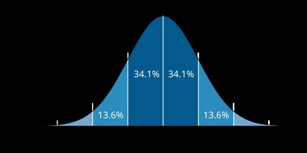Posterior Distribution Mode and Median

Image: A visual representation of a normal distribution highlighting the mode and median, illustrating their relationship in symmetrical data.

7. Case Studies: Real-World Examples

To further illustrate the practical differences, let’s delve into specific case studies where the choice between posterior mode and median has significant implications.

7.1. Case Study 1: Estimating Disease Prevalence

Consider a scenario where health officials want to estimate the prevalence of a rare disease in a population. They collect data from a sample of individuals and use a Bayesian model to estimate the prevalence rate. The posterior distribution of the prevalence rate is skewed due to the rarity of the disease.

Using Posterior Mode: The posterior mode would provide the single most likely estimate of the prevalence rate. This could be useful for setting public health policies and allocating resources. However, due to the skewness of the distribution, the mode might underestimate the true prevalence rate.
Using Posterior Median: The posterior median would provide a more robust estimate of the prevalence rate, less sensitive to the skewness of the distribution. This would give a more balanced and accurate view, crucial for planning effective interventions and understanding the disease’s impact.

7.2. Case Study 2: Predicting Financial Market Volatility

In finance, predicting market volatility is critical for risk management and investment strategies. A Bayesian model can be used to estimate the volatility of a stock based on historical data. The posterior distribution of the volatility parameter often has heavy tails and is sensitive to extreme market events.

Using Posterior Mode: The posterior mode would identify the most likely volatility level. This could be used for short-term trading strategies. However, in volatile markets, relying solely on the mode could lead to underestimating risk.
Using Posterior Median: The posterior median would offer a more stable measure of typical volatility, smoothing out the impact of extreme events. This would provide a more conservative estimate, better suited for long-term investment decisions and risk assessment.

7.3. Case Study 3: Optimizing Manufacturing Processes

In manufacturing, optimizing process parameters is essential for improving product quality and efficiency. A Bayesian model can be used to estimate the optimal settings for these parameters. The posterior distribution might be multimodal due to complex interactions between the parameters.

Using Posterior Mode: The posterior mode could identify the single best setting, assuming unimodality. However, in a multimodal scenario, it would only capture one of the possible optimal settings, potentially missing better alternatives.
Using Posterior Median: The posterior median would provide a compromise setting, representing the “middle ground” across the different modes. This might not be the absolute best setting, but it would offer a more reliable starting point for further optimization.

8. Advanced Techniques and Considerations

Beyond the basic definitions and applications, there are advanced techniques and considerations that can enhance the use of posterior mode and median.

8.1. Bayesian Model Averaging

Bayesian Model Averaging (BMA) is a technique for combining the results of multiple models to improve predictive accuracy and reduce model uncertainty. Instead of relying on a single model, BMA averages the posterior distributions from different models, weighted by their posterior probabilities.

Application: In situations where there are multiple plausible models, BMA can be used to obtain a more robust estimate of the posterior mode or median. This involves computing the posterior mode or median for each model and then averaging these estimates, weighted by the posterior probabilities of the models.

8.2. Hierarchical Bayesian Models

Hierarchical Bayesian models are used to model complex data structures with multiple levels of nesting. These models allow for the sharing of information across different levels of the hierarchy, improving the accuracy and efficiency of the estimates.

Application: In hierarchical models, the posterior mode and median can be computed at each level of the hierarchy. This allows for the estimation of parameters at different levels of aggregation, providing a more comprehensive understanding of the data.

8.3. Sensitivity Analysis

Sensitivity analysis involves assessing the sensitivity of the results to changes in the prior distribution or model assumptions. This is important for ensuring the robustness of the conclusions and identifying potential sources of bias.

Application: The posterior mode and median can be used to conduct sensitivity analysis. By varying the prior distribution or model assumptions and observing how the posterior mode and median change, one can assess the sensitivity of the results and identify potential sources of bias.

9. Tools and Software for Calculation

Calculating the posterior mode and median often requires specialized software. Here are some popular tools:

R: With packages like rstan, rjags, and MCMCpack, R provides extensive capabilities for Bayesian analysis, including functions to compute posterior mode and median using MCMC sampling.
Python: Libraries such as PyMC3 and Stan offer similar functionalities to R, allowing for flexible model specification and posterior inference.
JAGS and Stan: These are standalone programs specifically designed for Bayesian computation using MCMC. They can be integrated with R and Python.

These tools streamline the process of Bayesian inference, enabling researchers to focus on model building and interpretation rather than computational details.

10. Common Pitfalls and How to Avoid Them

While the posterior mode and median are valuable measures, there are common pitfalls to avoid:

Misinterpreting the Mode in Multimodal Distributions: Ensure that the mode identified is the global mode and not a local one. Use visualization tools to understand the shape of the posterior distribution.
Ignoring Skewness: In highly skewed distributions, the mode might not be representative. Always consider the median and other quantiles to get a complete picture.
Over-Reliance on Default Priors: The choice of prior can significantly impact the posterior. Conduct sensitivity analyses to assess the impact of different priors.
Computational Errors: Ensure that the MCMC chains have converged and that the optimization algorithms have found the true mode. Check convergence diagnostics and perform multiple runs.

By being aware of these potential issues and taking steps to address them, analysts can ensure the reliability and validity of their Bayesian inferences.

Image: A visual representation comparing the mean, median, and mode in various distributions, emphasizing the impact of skewness on their relative positions.

11. Future Trends in Bayesian Statistics

Bayesian statistics is a rapidly evolving field, with new methods and applications emerging constantly. Some future trends include:

Increased Use of Machine Learning Techniques: Combining Bayesian methods with machine learning algorithms for improved prediction and inference.
Scalable Bayesian Computation: Developing more efficient algorithms for handling large datasets and complex models.
Automated Bayesian Modeling: Creating tools and techniques for automating the process of model selection and inference.
Bayesian Deep Learning: Integrating Bayesian principles into deep learning models for improved uncertainty quantification and robustness.

These trends promise to further enhance the power and applicability of Bayesian statistics in various domains.

12. Conclusion: Choosing the Right Measure for Your Analysis

In summary, both the posterior mode and median provide valuable insights into the posterior distribution, but they do so in different ways. The posterior mode represents the most likely value and is useful for decision-making, while the posterior median provides a more robust and balanced estimate, less sensitive to extreme values and skewness.

Choosing between the posterior mode and median depends on the specific characteristics of the posterior distribution and the goals of the analysis. If the posterior distribution is approximately symmetric and unimodal, the mode and median will be similar, and either measure can be used. However, if the posterior distribution is skewed or has heavy tails, the median is generally preferred.

Ultimately, the best approach is to consider both measures, along with other features of the posterior distribution, to gain a comprehensive understanding of the parameter of interest.

Are you struggling to compare different statistical measures for your data analysis? Visit COMPARE.EDU.VN today to access detailed comparisons, expert reviews, and user feedback, and make informed decisions. Our comprehensive resources will help you navigate the complexities of statistical analysis with ease. Contact us at 333 Comparison Plaza, Choice City, CA 90210, United States or reach out via Whatsapp at +1 (626) 555-9090. Explore more at compare.edu.vn and start making smarter comparisons today!

13. FAQ Section

Here are some frequently asked questions about posterior mode and median:

1. What is the posterior distribution?

The posterior distribution combines prior beliefs with evidence from observed data, representing updated knowledge about a parameter.

2. How does the posterior mode differ from the posterior mean?

The posterior mode is the most likely value, while the posterior mean is the average value. In skewed distributions, they can differ significantly.

3. When should I use the posterior mode?

Use the posterior mode when you need a single, most likely estimate for decision-making, especially with symmetric distributions.

4. Why is the posterior median more robust than the posterior mean?

The posterior median is less sensitive to extreme values and skewness, providing a more balanced representation.

5. What are the limitations of the posterior mode in multimodal distributions?

The mode may not be unique and requires identifying the global mode, which can be challenging.

6. Can the choice of prior distribution affect the posterior mode and median?

Yes, the prior can influence both measures, but the mode is generally more sensitive to the prior than the median.

7. How do I calculate the posterior mode and median for complex distributions?

Use numerical methods like MCMC sampling, optimization algorithms, or integration techniques with software like R, Python, JAGS, or Stan.

8. What is Bayesian Model Averaging (BMA), and how does it relate to the posterior mode and median?

BMA combines results from multiple models to improve accuracy, averaging the posterior distributions and their respective mode or median estimates.

9. How can sensitivity analysis help in Bayesian inference?

Sensitivity analysis assesses how changes in the prior or model assumptions affect the results, ensuring robustness.

10. What are the future trends in Bayesian statistics that I should be aware of?

Future trends include increased use of machine learning, scalable computation, automated modeling, and Bayesian deep learning.