The American Community Survey (ACS) provides valuable data on various demographic and socioeconomic characteristics. A common question is how to compare ACS estimates, particularly over time, and how they relate to decennial census data. This article delves into the complexities of comparing ACS data, focusing on key considerations and providing practical examples using formulas and maps.
Key Considerations When Comparing ACS Estimates
Several factors complicate direct comparisons of ACS estimates:
-
Period Estimates: The ACS publishes 1-year and 5-year estimates. One-year estimates are limited to areas with populations over 65,000. For smaller geographies like census tracts, 5-year estimates are necessary. Crucially, only non-overlapping 5-year periods should be compared (e.g., 2015-2019 vs. 2010-2014) to avoid using the same data multiple times.
-
Changing Geography: Census boundaries are updated every ten years following the decennial census. This means comparing data across decades requires careful consideration of boundary changes. Tracts can be split, merged, or renumbered, making direct comparisons challenging. Using normalized census data can help address this issue but requires additional effort.
-
Margins of Error: All ACS estimates have margins of error, reflecting the survey’s sample-based nature. These margins are crucial when comparing estimates. Small differences might be due to random sampling variability rather than actual change, especially in smaller geographies or for smaller population subgroups. Statistical significance tests are necessary to determine if observed differences are real.
Formulas for Comparing ACS Estimates
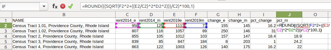
Let’s illustrate with an example comparing median gross rent in Providence County, Rhode Island, between the 2014 (2010-2014) and 2019 (2015-2019) 5-year ACS estimates.
1. Change and Percent Change:
- Change: Subtract the earlier estimate from the later estimate (Est2 – Est1).
- Percent Change: Divide the change by the earlier estimate and multiply by 100:
((Est2 - Est1) / Est1) * 100.
2. Margin of Error for Change and Percent Change:
- Change MOE:
SQRT((Est1_MOE^2) + (Est2_MOE^2)). - Percent Change MOE:
((SQRT(Est2_MOE^2 + ((Est2/Est1)^2 * Est1_MOE^2))) / Est1) * 100. This formula accounts for the ratio nature of percent change.
3. Coefficient of Variation (CV): Indicates the reliability of the change estimate:
- CV:
ABS((Est_MOE / 1.645) / Est) * 100. Values below 12 indicate high reliability, 13-34 medium, and above 35 low. (Note: This is a conservative range).
4. Test for Statistical Difference: Determines if the difference is statistically significant:
- Significant Difference:
ABS((Est2 - Est1) / (SQRT((Est1_MOE / 1.645)^2 + (Est2_MOE / 1.645)^2))). A value greater than 1.645 indicates a statistically significant difference at the 90% confidence level.
Mapping the Results: Visualizing Change and Significance
Mapping statistically significant changes alongside their reliability (CV) provides a powerful visual representation of true change.
Mapping only statistically significant changes paints a more accurate picture, filtering out noise due to sampling variability. Further classifying these changes by their reliability (CV) highlights areas where even significant change might be measured with low precision.
Conclusion
Comparing ACS data requires careful consideration of period estimates, geographic changes, and margins of error. Using formulas to calculate change, percent change, margins of error, coefficients of variation, and statistical significance is essential. Mapping these results enhances understanding by visually representing true change and its reliability. Remember to adjust for inflation when comparing dollar values over time and consider using decennial census data for basic demographic information when appropriate. For more in-depth guidance, consult the Census Bureau’s resources on comparing ACS data. Always prioritize careful interpretation and acknowledge limitations when working with ACS estimates.