Can I Compare Logit To Linear Regression Model? Absolutely. COMPARE.EDU.VN provides an in-depth analysis, highlighting the differences, advantages, and disadvantages of each model to help you choose the most suitable approach for your data. Discover the nuances of predictive modeling and make informed decisions with comprehensive statistical analysis.
1. Understanding Linear and Logit Regression Models
When dealing with a dichotomous outcome variable, such as success or failure, yes or no, a crucial decision arises: can I compare logit to linear regression model? Linear regression, in its simplicity, models the probability directly as a linear function of the predictors. Logit regression, on the other hand, models the natural logarithm of the odds of the outcome as a linear function of the predictors. The choice between these models hinges on several factors, including interpretability, model fit, and the range of probabilities being modeled.
The key distinction lies in how each model treats the dependent variable. Linear regression assumes a linear relationship between the predictors and the probability of the outcome, while logit regression uses a logistic function to ensure that predicted probabilities remain within the 0 to 1 range. This difference has significant implications for the interpretation and applicability of each model. Understanding these foundational aspects is crucial for making an informed decision when choosing between logit and linear regression.
2. Interpretability: A Key Advantage of Linear Regression
One of the most compelling reasons to consider using a linear probability model is its straightforward interpretability. In a linear regression, the coefficient associated with a predictor variable represents the change in the probability of the outcome variable for a one-unit increase in the predictor, holding all other variables constant. This interpretation is intuitive and easy to communicate, making it particularly useful in fields where clear explanations are paramount.
For instance, if a coefficient for an education variable in a linear probability model is 0.05, it means that each additional year of education is associated with a 5 percentage point increase in the probability of a positive outcome. This directness is invaluable for policymakers, stakeholders, and anyone else who needs to understand the impact of different factors on the outcome of interest.
3. Decoding the Logit Model: Odds, Log-Odds, and Interpretation Challenges
The logit model, while powerful, presents challenges in interpretation. The coefficients in a logit model represent the change in the log-odds of the outcome variable for a one-unit increase in the predictor, which is not immediately intuitive. To make the results more understandable, researchers often convert log-odds to odds ratios by exponentiating the coefficients.
Even with odds ratios, interpretation can be tricky. An odds ratio of 2, for example, means that a one-unit increase in the predictor doubles the odds of the outcome occurring. However, the impact on the probability depends on the baseline probability. Doubling the odds from 0.1 to 0.2 results in a smaller change in probability than doubling the odds from 0.5 to 1. This complexity makes it harder to grasp the practical implications of the results compared to the straightforward interpretation of linear regression.
4. Odds Ratios: A Closer Look at Their Intuition (or Lack Thereof)
While odds ratios are commonly used to interpret logit models, their intuitive appeal is often overstated. People tend to confuse odds with probabilities, leading to misinterpretations. For example, if a get-out-the-vote campaign doubles the odds of voting, it does not mean that a person’s probability of voting doubles. The actual change in probability depends on the initial probability.
Consider someone with a baseline probability of voting of 40%. Doubling their odds of 0.67 results in new odds of 1.33, which translates to a probability of approximately 57%. This difference highlights the need for careful calculation and a clear understanding of the distinction between odds and probabilities. The complexity of interpreting odds ratios can be a significant drawback, especially when communicating results to a non-technical audience.
5. The Nonlinearity of the Logit Model: When Does It Matter?
The logit model is inherently nonlinear, which can be both an advantage and a disadvantage. The logistic function ensures that predicted probabilities always fall between 0 and 1, avoiding the possibility of out-of-bounds predictions that can occur with linear regression. However, the nonlinearity also means that the relationship between the predictors and the outcome is not constant across the range of probabilities.
The importance of the nonlinearity depends on the range of probabilities being modeled. If the probabilities are mostly between 0.2 and 0.8, the relationship between the probability and the log-odds is approximately linear. In such cases, a linear regression can provide a good approximation to the logit model, with the added benefit of easier interpretation. However, when probabilities are close to 0 or 1, the nonlinearity becomes more pronounced, and the logit model is generally more appropriate.
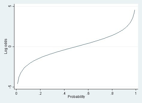 Nonlinear relationship between probability and log odds
6. A Practical Guideline: When to Choose Linear vs. Logit Regression
A useful rule of thumb is to consider the range of probabilities being modeled. If the probabilities are mostly between 0.2 and 0.8, a linear regression model can be a reasonable choice, offering simplicity and interpretability. However, if the probabilities extend to the extremes, approaching 0 or 1, a logit model is generally preferred to ensure accurate predictions and avoid out-of-bounds values.
For example, when modeling the probability of voting or being overweight, where the probabilities for most individuals fall within the 0.2 to 0.8 range, a linear probability model can be a good fit. On the other hand, when modeling rare events, such as the probability of a bank transaction being fraudulent, where the probabilities are typically very low, a logit model is more appropriate.
7. Extreme Probabilities: The Achilles Heel of Linear Regression
The primary weakness of linear regression when modeling dichotomous outcomes is its susceptibility to producing predicted probabilities that fall outside the valid range of 0 to 1. This issue arises because linear regression does not constrain the predicted values to be within these bounds. When the true probabilities are close to 0 or 1, the linear model can easily generate predictions that are negative or greater than 1, which are nonsensical.
These out-of-bounds predictions can lead to misleading conclusions and undermine the credibility of the model. While there are methods to truncate or adjust the predictions to fall within the valid range, these adjustments can introduce bias and distort the results. The logit model, by design, avoids this problem, making it a more reliable choice when dealing with extreme probabilities.
8. Logit Regression and Rare Events: Addressing Potential Biases
While logit regression is generally preferred for modeling rare events, it is not without its challenges. When dealing with very low probabilities, logit models can suffer from issues such as complete separation, quasi-complete separation, and rare events bias. These problems can lead to inflated coefficient estimates and unreliable predictions.
Complete separation occurs when a predictor variable perfectly predicts the outcome, resulting in infinite coefficient estimates. Quasi-complete separation occurs when a predictor variable almost perfectly predicts the outcome, leading to very large coefficient estimates. Rare events bias arises when the outcome is very rare, leading to biased coefficient estimates. Several remedies are available to address these issues, including using penalized regression techniques or adjusting the estimation procedure.
9. Computational Efficiency: The Speed Advantage of Linear Regression
In addition to interpretability, linear regression offers a significant advantage in terms of computational efficiency. Fitting a linear regression model is typically much faster than fitting a logit model, especially for large datasets or complex models. Linear regression can be estimated non-iteratively using ordinary least squares (OLS), while logit regression requires an iterative process of maximum likelihood estimation.
The speed difference can be substantial, particularly when working with massive datasets or computationally intensive models. In some cases, switching from a logit model to a linear probability model can reduce the runtime from days to hours, making it a practical consideration when computational resources are limited.
10. Heteroscedasticity in Linear Probability Models: A Minor Concern
One potential concern with using linear regression to model dichotomous outcomes is heteroscedasticity, which means that the variance of the errors is not constant across all observations. In a linear probability model, the residual variance is given by p(1-p), where p is the predicted probability. This variance is highest when p is close to 0.5 and lowest when p is close to 0 or 1.
However, the impact of heteroscedasticity is often minor, especially when the probabilities are mostly between 0.2 and 0.8. In such cases, the OLS estimates are still unbiased, although the standard errors may be inaccurate. To address this issue, researchers can use heteroscedasticity-consistent standard errors or weighted least squares, although these improvements often make little difference in practice.
11. Real-World Applications: Examples of Linear and Logit Regression Use
To illustrate the practical application of linear and logit regression, consider a few real-world examples. In marketing, a linear probability model might be used to predict the probability of a customer making a purchase based on their demographics and browsing history. In this case, the probabilities are likely to fall within a moderate range, making linear regression a reasonable choice.
On the other hand, in fraud detection, a logit model might be used to predict the probability of a transaction being fraudulent. Because fraudulent transactions are rare, the probabilities are typically very low, making logit regression the more appropriate choice. Similarly, in medical research, a logit model might be used to predict the probability of a patient developing a disease based on their risk factors.
12. Model Fit: Assessing How Well Each Model Explains the Data
Model fit is a critical consideration when choosing between linear and logit regression. Several metrics can be used to assess how well each model explains the data, including the R-squared, the Akaike Information Criterion (AIC), and the Bayesian Information Criterion (BIC). The R-squared measures the proportion of variance in the dependent variable that is explained by the model, with higher values indicating a better fit.
The AIC and BIC are information criteria that balance model fit with model complexity, with lower values indicating a better fit. In general, the model with the best fit, as indicated by these metrics, should be preferred. However, it is important to consider the interpretability and computational efficiency of each model as well.
13. Beyond the Basics: Advanced Techniques and Considerations
In some cases, neither linear nor logit regression may be the ideal choice. When dealing with complex relationships or non-linear effects, more advanced techniques may be necessary. These techniques include generalized additive models (GAMs), neural networks, and support vector machines (SVMs). GAMs allow for non-linear relationships between the predictors and the outcome, while neural networks and SVMs can model highly complex patterns in the data.
However, these advanced techniques often come at the cost of increased complexity and reduced interpretability. It is important to carefully weigh the benefits of improved model fit against the drawbacks of increased complexity when choosing a modeling approach.
14. Addressing Overfitting: Balancing Complexity and Generalization
Overfitting is a common problem in statistical modeling, particularly when using complex models with many predictors. Overfitting occurs when a model fits the training data too well, capturing noise and random variation rather than the underlying relationships. This can lead to poor performance on new, unseen data.
To address overfitting, several techniques can be used, including regularization, cross-validation, and model simplification. Regularization adds a penalty term to the model objective function, discouraging overly complex models. Cross-validation involves splitting the data into multiple subsets and using each subset to evaluate the model’s performance. Model simplification involves reducing the number of predictors or using a simpler functional form.
15. Interaction Effects: Modeling Complex Relationships Between Variables
Interaction effects occur when the relationship between a predictor variable and the outcome variable depends on the value of another predictor variable. For example, the effect of education on income may depend on gender, with education having a larger effect for men than for women. Modeling interaction effects can improve the accuracy and interpretability of the model.
To model interaction effects, interaction terms can be added to the regression equation. An interaction term is created by multiplying two predictor variables together. The coefficient associated with the interaction term represents the change in the effect of one predictor variable on the outcome variable for a one-unit increase in the other predictor variable.
16. Non-Linear Relationships: Transforming Predictor Variables
In some cases, the relationship between a predictor variable and the outcome variable may be non-linear. For example, the effect of age on health outcomes may be non-linear, with health declining more rapidly in older age. In such cases, transforming the predictor variable can improve the fit of the model.
Common transformations include taking the logarithm, square root, or square of the predictor variable. The choice of transformation depends on the nature of the non-linearity. It is important to carefully consider the interpretability of the transformed variable when choosing a transformation.
17. The Importance of Data Quality: Garbage In, Garbage Out
The quality of the data is crucial for the success of any statistical modeling effort. If the data is inaccurate, incomplete, or inconsistent, the results of the model will be unreliable. It is important to carefully clean and preprocess the data before building the model.
Data cleaning involves identifying and correcting errors, inconsistencies, and missing values. Preprocessing involves transforming the data into a suitable format for the model. This may include scaling the variables, creating dummy variables, or handling outliers.
18. Ethical Considerations: Avoiding Bias and Discrimination
Statistical models can perpetuate bias and discrimination if they are not used carefully. It is important to be aware of potential sources of bias in the data and to take steps to mitigate them. For example, if the data contains biased samples, the model may produce biased predictions.
To avoid bias and discrimination, it is important to use representative data, to carefully consider the choice of predictors, and to evaluate the model’s performance across different subgroups. It is also important to be transparent about the limitations of the model and to avoid using it for purposes that could harm individuals or groups.
19. Communicating Results Effectively: Visualizations and Explanations
Communicating the results of a statistical model effectively is essential for ensuring that the findings are understood and used appropriately. Visualizations, such as graphs and charts, can be a powerful tool for conveying complex information in a clear and concise manner.
Explanations should be tailored to the audience, avoiding technical jargon and focusing on the practical implications of the results. It is important to be honest about the limitations of the model and to avoid overstating the conclusions.
20. COMPARE.EDU.VN: Your Partner in Data-Driven Decision Making
Navigating the complexities of statistical modeling can be challenging. At COMPARE.EDU.VN, we provide comprehensive comparisons and resources to help you make informed decisions about the best analytical approaches for your needs. Whether you’re comparing logit to linear regression or exploring other advanced techniques, our goal is to empower you with the knowledge and tools you need to succeed.
We understand the challenges you face when comparing different options, the difficulty in finding objective and detailed information, the confusion caused by information overload, and the need for clear and intuitive comparisons. Our platform is designed to address these challenges by providing detailed comparisons, highlighting pros and cons, comparing features and prices, and offering user reviews and expert opinions.
FAQ: Linear Regression vs. Logit Models
1. What is the main difference between linear and logit regression?
Linear regression models the probability directly, while logit regression models the natural logarithm of the odds of the outcome.
2. When should I use linear regression instead of logit regression?
Use linear regression when the probabilities are mostly between 0.2 and 0.8 and interpretability is a priority.
3. What are the advantages of using a logit model?
Logit models ensure that predicted probabilities remain within the 0 to 1 range and are more appropriate for extreme probabilities.
4. How do I interpret the coefficients in a logit model?
Coefficients in a logit model represent the change in the log-odds of the outcome variable for a one-unit increase in the predictor.
5. What is an odds ratio, and how is it calculated?
An odds ratio is the exponentiated coefficient in a logit model, representing the change in the odds of the outcome for a one-unit increase in the predictor.
6. What are the potential problems with using linear regression for dichotomous outcomes?
Linear regression can produce predicted probabilities that fall outside the valid range of 0 to 1.
7. How does heteroscedasticity affect linear probability models?
Heteroscedasticity can lead to inaccurate standard errors in linear probability models, but the impact is often minor when probabilities are between 0.2 and 0.8.
8. What is rare events bias, and how does it affect logit models?
Rare events bias occurs when the outcome is very rare, leading to biased coefficient estimates in logit models.
9. How can I address overfitting in statistical models?
Techniques to address overfitting include regularization, cross-validation, and model simplification.
10. What are interaction effects, and how are they modeled in regression?
Interaction effects occur when the relationship between a predictor variable and the outcome variable depends on the value of another predictor variable.
Take the Next Step with COMPARE.EDU.VN
Ready to make informed decisions? Visit COMPARE.EDU.VN today to explore detailed comparisons, expert reviews, and user insights. Our comprehensive resources will help you evaluate your options and choose the best solutions for your unique needs.
Address: 333 Comparison Plaza, Choice City, CA 90210, United States
Whatsapp: +1 (626) 555-9090
Website: COMPARE.EDU.VN
Let compare.edu.vn guide you to smarter choices and better outcomes.