How To Compare 2 Columns And Remove Duplicates In Excel?

Are you looking for a way to compare two columns in Excel and remove duplicates? COMPARE.EDU.VN provides a guide to help you identify and manage duplicate data. This involves using formulas or specialized tools to highlight, remove, or list duplicate entries. Improve data accuracy and efficiency by following this process. Discover how to compare data, delete duplicate rows, and use conditional formatting in this comprehensive guide.

1. What Are The Ways To Compare 2 Columns In Excel To Find Duplicates Using Excel Formulas?

To compare two columns for duplicates using Excel formulas, you can use the MATCH and IF functions. This method involves creating a formula that checks if a value in one column exists in another, flagging duplicates accordingly.

Here’s how to do it:

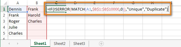
Variant A: Columns on the same sheet
1. In an empty cell (e.g., C1), enter the following formula:
  =IF(ISERROR(MATCH(A1,$B$1:$B$10000,0)),"Unique","Duplicate")
  - A1: The first cell in the first column to compare.
  - $B$1:$B$10000: The range of cells in the second column to compare against. The dollar signs create an absolute cell reference, preventing the cell range from changing when copying the formula.
2. Copy the formula down to all the cells in column C, corresponding to the data in column A. To do this quickly, select cell C1, click the small square at the bottom-right corner, and drag it down. For large tables, copy cell C1 (Ctrl + C), select the range (Ctrl + Shift + End), and paste (Ctrl + V).
3. Column C will now flag each entry in column A as “Duplicate” if it exists in column B, or “Unique” if it doesn’t.
Variant B: Columns on different worksheets
1. In the first cell of an empty column in Sheet2 (e.g., column B), enter the following formula:
  =IF(ISERROR(MATCH(A1,Sheet3!$A$1:$A$10000,0)),"","Duplicate")
  - A1: The first cell in the first column of Sheet2.
  - Sheet3!$A$1:$A$10000: The range of cells in column A of Sheet3 to compare against.
2. Copy the formula down as described in Variant A.
3. The column in Sheet2 will flag duplicates found in Sheet3.

2. How Can I Work With Found Duplicates After Comparing Two Columns In Excel?

Once you’ve identified duplicates in Excel using formulas, the next step is to manipulate this data. You can show only duplicated rows, color-highlight them, or remove them, depending on your goal.

Show only duplicated rows:
1. Add headers to your columns if they don’t already have them. Insert a new row at the top (right-click the row number and select “Insert”). Name the columns (e.g., “Name” and “Duplicate?”).
2. Apply a filter to your data. Go to the “Data” tab and click “Filter.”
3. Click the arrow next to the “Duplicate?” column header.
4. In the drop-down menu, uncheck “Unique” and click “OK”. Only the rows flagged as “Duplicate” will be visible.
5. To revert the filter, click the filter icon in the “Duplicate?” column, then click “Select All” or go to “Data” > “Sort & Filter” > “Clear.”
Color or highlight found duplicates:
1. Filter for duplicates as described above.
2. Select all the visible cells containing duplicates.
3. Press Ctrl + 1 to open the “Format Cells” dialog box.
4. Go to the “Fill” tab and choose a background color to highlight the duplicates.
5. Click “OK.” The duplicated cells will now be highlighted with the color you selected.
Remove duplicates from the first column:
- If the columns are on different worksheets:
  1. Filter the table to show only rows with duplicates.
  2. Select the visible rows.
  3. Right-click the selected range and choose “Delete Row.”
  4. Confirm the deletion and clear the filter.
- If the columns are on the same worksheet:
  1. Filter the table to show only duplicated cells and select those cells.
  2. Right-click the selection and choose “Clear Contents” to remove the values.
  3. Clear the filter.
  4. Select all cells in the first column from the top to the last data entry.
  5. Go to the “Data” tab and click “Sort A to Z”.
  6. In the sort dialog box, select “Continue with the current selection” and click “Sort.” This will move the cleared (empty) cells to the top.
  7. Delete the column containing the formula, as it’s no longer needed.

3. How Can I Use The Visual Wizard To Compare 2 Excel Columns For Duplicates?

A visual wizard can greatly simplify the process of comparing columns and removing duplicates in Excel. Tools like Ablebits’ Dedupe tools provide a user-friendly interface to handle this task efficiently.

Here’s how to use such a wizard:

Install and open the add-in:
- Install the Ablebits Ultimate Suite for Excel.
- Open the Excel worksheet where your columns are located.
Select the data range:
- Select any cell within the first column you want to compare.
- Go to the “Ablebits Data” tab and click the “Compare Tables” button.
Specify the columns to compare:
- The wizard will automatically select the first column. Click “Next.” If you’re comparing entire tables, select the whole table.
- On the second step, select the second column to compare against. The wizard often auto-selects this; if not, manually select the column or table.
Choose the comparison type:
- Select “Duplicate values” to find entries that appear in both columns.
Select the columns pairs for comparison:
- Choose the specific pairs of columns you want to compare. This is particularly useful when comparing multiple columns across two tables.
Choose what to do with the found duplicates:
- You can opt to delete, move, highlight, or select the duplicate entries. For safety, especially when using the tool for the first time, choose to move duplicates to another worksheet. This lets you review the identified duplicates before permanently removing them.
Finish the process:
- Click “Finish” to execute the comparison and action. The wizard will then perform the selected action, such as moving the duplicates to a new sheet, highlighting them, or removing them from the original data.

4. What Are The Benefits Of Using Excel Formulas To Compare Two Columns?

Using Excel formulas to compare two columns offers several benefits, especially in scenarios where you need a dynamic and customizable solution.

Customization: Formulas allow you to tailor the comparison criteria to your specific needs. You can modify the logic to find exact matches, partial matches, or even use more complex conditions.
No additional software: Formulas are built into Excel, so you don’t need to install any extra add-ins or software.
Dynamic results: Formulas automatically update whenever the data in your columns changes. This ensures that your comparison results are always current.
Learning opportunity: Working with formulas helps you improve your Excel skills and understand how to manipulate data effectively.
Transparency: Formulas are visible in the worksheet, so you can easily see and understand the logic behind the comparison.
Flexibility: You can combine formulas with other Excel features like conditional formatting or data validation to create powerful data analysis tools.

5. What Are The Limitations Of Using Excel Formulas To Compare Two Columns?

While using Excel formulas for comparing columns is beneficial, there are also limitations to consider:

Complexity: Writing and understanding formulas can be complex, especially for users who are not familiar with Excel functions like MATCH, IF, ISERROR, and others.
Time-consuming: Manually writing and copying formulas across a large dataset can be time-consuming.
Error-prone: It’s easy to make mistakes when writing formulas, which can lead to inaccurate results. Double-checking and testing are crucial.
Performance: For very large datasets, formulas can slow down Excel, impacting performance and responsiveness.
Maintenance: If your data structure changes, you may need to update your formulas, which can be cumbersome.
Lack of advanced features: Formulas do not offer the advanced features that dedicated tools provide, such as fuzzy matching or automated data cleaning.

6. How Does Conditional Formatting Help In Comparing Two Columns In Excel?

Conditional formatting in Excel provides a visual way to compare two columns, highlighting differences or matches based on specified criteria. This can make it easier to identify patterns or discrepancies in your data.

Here’s how conditional formatting can be used for comparing columns:

Select the range: Choose the range of cells in the first column you want to compare.
Open conditional formatting:
- Go to the “Home” tab in Excel.
- Click on “Conditional Formatting” in the “Styles” group.
Create a new rule:
- Select “New Rule…” from the drop-down menu.
- Choose “Use a formula to determine which cells to format.”
Enter the formula:
- Enter a formula that compares the selected cell in the first column with the corresponding cell in the second column. For example, to highlight matches:
  =A1=B1
  To highlight differences:
  =A1<>B1
  Where A1 is the first cell in the first column and B1 is the first cell in the second column.
Set the format:
- Click the “Format…” button.
- Choose the formatting style you want to apply (e.g., fill color, font color, borders).
- Click “OK” to set the format.
Apply the rule:
- Click “OK” in the “New Formatting Rule” dialog to apply the conditional formatting.

7. When Is It Better To Use A Dedicated Excel Add-In Instead Of Formulas For Comparing Columns?

Deciding between using a dedicated Excel add-in and formulas for comparing columns depends on the complexity of the task and your comfort level with Excel functions. Add-ins like Ablebits Ultimate Suite are particularly useful in certain situations:

Large Datasets: Add-ins are optimized to handle large datasets more efficiently than formulas, reducing the risk of Excel slowing down or crashing.
Complex Comparisons: If you need to perform complex comparisons, such as fuzzy matching or comparing multiple criteria, add-ins offer more advanced features that are difficult to replicate with formulas.
User-Friendly Interface: Add-ins provide a user-friendly interface that simplifies the comparison process, making it easier for users who are not familiar with Excel formulas.
Automated Tasks: Add-ins often include automated tasks, such as data cleaning and formatting, which can save you time and effort.
Regular Use: If you frequently compare columns in Excel, an add-in can streamline the process and improve your productivity.
Advanced Features: Add-ins may offer features such as side-by-side comparison views, detailed reporting, and the ability to undo changes, which are not available with formulas.

8. Can I Compare More Than Two Columns At Once In Excel?

Yes, you can compare more than two columns at once in Excel, although the method you use might differ depending on whether you are using formulas or a dedicated add-in.

Using Formulas: Comparing multiple columns with formulas can become complex but is achievable. You can extend the MATCH and IF formula approach to include multiple columns. For example, to check if a value in column A exists in columns B, C, and D, you would nest multiple MATCH functions within an IF function. This approach can become cumbersome and difficult to manage as the number of columns increases.
Using Add-Ins: Dedicated Excel add-ins like Ablebits Ultimate Suite are designed to handle multi-column comparisons more efficiently. These add-ins typically allow you to select multiple columns for comparison and provide options for finding duplicates, unique values, or differences across the selected columns. The add-ins often offer a user-friendly interface that simplifies the process of selecting columns and defining comparison criteria.

9. How Do I Handle Errors When Comparing Columns With Formulas In Excel?

When comparing columns with formulas in Excel, errors can occur due to various reasons, such as mismatched data types, incorrect cell references, or values not found. Handling these errors gracefully is essential to ensure accurate and reliable results.

Using IFERROR Function: The IFERROR function is useful for catching and handling errors in Excel formulas. It allows you to specify a value to return if a formula evaluates to an error. For example, if the MATCH function returns an error because a value is not found, you can use IFERROR to display a custom message or a blank value.
Checking Data Types: Ensure that the data types in the columns you are comparing are consistent. Mismatched data types (e.g., comparing text with numbers) can lead to errors. Use functions like ISTEXT, ISNUMBER, and ISBLANK to check data types and handle them accordingly.
Using Absolute and Relative References Correctly: Make sure that you are using absolute ($) and relative references correctly in your formulas. Absolute references are used to lock cell references, while relative references change as you copy the formula. Incorrect use of references can lead to formulas comparing the wrong cells.
Validating Input Data: Before comparing columns, validate the input data to ensure that it meets the expected criteria. Use data validation rules to restrict the type of data that can be entered in a cell, such as numbers, dates, or text.
Using Helper Columns: Create helper columns to break down complex formulas into smaller, more manageable steps. This can make it easier to identify and fix errors.

10. What Are Some Best Practices For Maintaining Data Integrity When Removing Duplicates In Excel?

Maintaining data integrity when removing duplicates in Excel is crucial to ensure that your data remains accurate and reliable. Here are some best practices to follow:

Back Up Your Data: Before removing any duplicates, always create a backup of your Excel file. This ensures that you can revert to the original data if something goes wrong.
Understand Your Data: Before removing duplicates, take the time to understand your data and identify the criteria for determining what constitutes a duplicate. Consider factors such as case sensitivity, leading or trailing spaces, and variations in data entry.
Use the Right Tools: Choose the right tools for removing duplicates based on the size and complexity of your data. For simple tasks, Excel’s built-in “Remove Duplicates” feature may be sufficient. For more complex tasks, consider using advanced filters, formulas, or dedicated add-ins.
Review Duplicates Before Removing: Whenever possible, review the duplicates identified by Excel before removing them. This allows you to verify that they are indeed duplicates and that you are not accidentally removing valid data.
Document Your Steps: Keep a record of the steps you take to remove duplicates, including the criteria used, the formulas applied, and the number of duplicates removed. This documentation can be helpful for auditing purposes and for replicating the process in the future.
Test Your Data: After removing duplicates, test your data to ensure that it is still accurate and complete. Check for any unexpected changes or errors and correct them as needed.

COMPARE.EDU.VN can help you compare data, delete duplicate rows, and use conditional formatting. You can visit us at 333 Comparison Plaza, Choice City, CA 90210, United States. Contact us via Whatsapp at +1 (626) 555-9090, or visit our website compare.edu.vn. Use our Excel guides to improve data accuracy and efficiency.

How To Compare 2 Columns And Remove Duplicates In Excel?

Comments

Leave a Reply Cancel reply