Comparing two columns in Excel for mismatches is a crucial skill for data analysis and validation. At COMPARE.EDU.VN, we offer a detailed guide on How To Compare Two Columns In Excel For Mismatches, identifying unique values, and ensuring data integrity. Learn effective techniques for mismatch detection using formulas, conditional formatting, and advanced Excel features. You’ll also discover how to highlight discrepancies and extract mismatched data, enhancing your spreadsheet proficiency with our comparison insights and data validation tools.
1. What Are the Search Intentions Behind “How to Compare Two Columns in Excel for Mismatches”?
Understanding the search intent behind the keyword “how to compare two columns in Excel for mismatches” helps tailor content to meet user needs effectively. Here are five common search intentions:
- Instructional Guides: Users seek step-by-step instructions on using Excel features and formulas to identify mismatched data between two columns.
- Formula Solutions: Individuals look for specific Excel formulas (e.g., COUNTIF, MATCH) to pinpoint mismatches and understand how these formulas work.
- Conditional Formatting: Users want to learn how to use conditional formatting to visually highlight mismatched data for easier identification.
- Data Validation Techniques: People search for methods to validate data integrity by comparing columns and ensuring consistency across datasets.
- Troubleshooting Assistance: Users look for solutions to common issues encountered while comparing columns, such as handling different data types or case sensitivity.
2. Comparing Two Columns in Excel Row by Row: Identifying Discrepancies
Comparing two columns row by row is essential for detailed data validation. Here’s how to use Excel’s IF function to highlight mismatches and ensure accuracy.
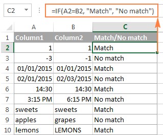
2.1. How Can I Use the IF Function to Compare Two Columns for Mismatches in the Same Row?
To compare two columns in Excel row by row, use the IF function to identify differences between corresponding cells. Enter the formula in a new column and drag it down to apply to all rows.
For example, if you want to compare column A and column B, the formula would be:
=IF(A2<>B2, "Mismatch", "")
This formula checks if the value in cell A2 is different from the value in cell B2. If they are different, it returns “Mismatch”; otherwise, it returns an empty string.
2.2. What Formula Can I Use to Identify Case-Sensitive Mismatches Between Two Columns?
To identify case-sensitive mismatches, use the EXACT function within an IF statement. The EXACT function checks if two text strings are identical, including case.
The formula is:
=IF(EXACT(A2, B2), "", "Mismatch")
This formula returns “Mismatch” if the text in cell A2 is not exactly the same as the text in cell B2 (including case); otherwise, it returns an empty string.
3. Comparing Multiple Columns for Mismatches: Advanced Techniques
When dealing with multiple columns, advanced techniques are necessary to efficiently identify mismatches and maintain data consistency.
3.1. How Can I Find Mismatches Across Multiple Columns in the Same Row?
To find mismatches across multiple columns, combine the AND function with the IF function. This checks if all specified conditions are true, indicating a match across all columns.
For instance, to compare columns A, B, and C, the formula is:
=IF(AND(A2=B2, B2=C2), "Match", "Mismatch")
This formula returns “Match” if all three cells (A2, B2, C2) have the same value; otherwise, it returns “Mismatch”. If any of the cells don’t match, it will highlight the mismatch.
3.2. How Do I Use COUNTIF to Identify Rows Where Not All Columns Match?
The COUNTIF function can determine if all columns in a row have matching values. By counting how many columns match the first column’s value, you can identify mismatches.
The formula is:
=IF(COUNTIF($A2:$E2, $A2)=5, "Match", "Mismatch")
In this formula, $A2:$E2 is the range of columns to compare, and 5 is the total number of columns. If the count equals the number of columns, it returns “Match”; otherwise, it returns “Mismatch,” highlighting any discrepancies.
4. Identifying Mismatches Between Two Columns: Comprehensive Methods
Identifying mismatches between two columns involves finding values present in one column but not in the other, ensuring data completeness and accuracy.
4.1. How Can I Use COUNTIF to Find Values in Column A That Are Not in Column B?
The COUNTIF function can identify values in column A that are not present in column B. By checking if the count of each value from column A in column B is zero, you can pinpoint mismatches.
The formula is:
=IF(COUNTIF($B:$B, $A2)=0, "Not in B", "")
This formula searches the entire column B for the value in cell A2. If the count is 0 (meaning the value is not found), it returns “Not in B”; otherwise, it returns an empty string. To improve performance on large datasets, specify a range instead of the entire column (e.g., $B$2:$B$100).
4.2. How Do I Use MATCH and ISERROR to Find Mismatches Between Two Columns?
The MATCH and ISERROR functions can also identify mismatches. MATCH finds the position of a value in a range, and ISERROR checks if the MATCH function returns an error, indicating the value is not found.
The formula is:
=IF(ISERROR(MATCH($A2, $B$2:$B$10, 0)), "Not in B", "")
This formula tries to find the value in cell A2 within the range $B$2:$B$10. If MATCH returns an error (meaning the value is not found), ISERROR returns TRUE, and the IF function returns “Not in B”; otherwise, it returns an empty string.
5. Extracting and Highlighting Mismatches: Visual and Practical Techniques
Extracting and highlighting mismatches makes it easier to review and correct data, ensuring accuracy and consistency across your datasets.
5.1. How Can I Highlight Mismatched Cells Using Conditional Formatting?
Conditional formatting can visually highlight mismatched cells. By creating a rule based on a formula, you can automatically shade cells that meet specific criteria.
To highlight mismatches, follow these steps:
- Select the cells you want to compare.
- Go to Conditional Formatting > New Rule > Use a formula to determine which cells to format.
- Enter the formula
=$A2<>$B2. - Click Format to choose a fill color.
- Click OK.
This will highlight cells in column A that do not match the corresponding cells in column B.
5.2. How Do I Extract a List of Mismatched Values From Two Columns?
To extract a list of mismatched values, use a combination of IF and ISNA functions with INDEX and MATCH. This dynamically creates a list of values from one column that are not found in the other.
Here’s the formula:
=IF(ISNA(MATCH(A2, $B$2:$B$10, 0)), A2, "")
Enter this formula in a new column and drag it down. It checks if each value in column A is found in the range $B$2:$B$10. If the value is not found (ISNA returns TRUE), the formula returns the value from column A; otherwise, it returns an empty string. You can then filter the column to display only the mismatched values.
6. Comparing Two Lists for Unique and Duplicate Entries
Comparing two lists often involves identifying unique entries (values present in only one list) and duplicate entries (values present in both lists).
6.1. How Do I Highlight Unique Entries in Two Columns?
To highlight unique entries in two columns, use conditional formatting with the COUNTIF function. This helps visually distinguish values that appear in only one of the columns.
For List 1 (column A), the formula is:
=COUNTIF($B$2:$B$10, $A2)=0
For List 2 (column B), the formula is:
=COUNTIF($A$2:$A$10, $B2)=0
Follow these steps for each column:
- Select the cells in the column.
- Go to Conditional Formatting > New Rule > Use a formula to determine which cells to format.
- Enter the appropriate formula.
- Click Format to choose a fill color.
- Click OK.
This will highlight unique values in each column, making them easy to identify.
6.2. How Can I Highlight Matching (Duplicate) Entries Between Two Columns?
To highlight matching entries between two columns, use conditional formatting with the COUNTIF function, setting the count greater than zero.
For List 1 (column A), the formula is:
=COUNTIF($B$2:$B$10, $A2)>0
For List 2 (column B), the formula is:
=COUNTIF($A$2:$A$10, $B2)>0
Follow these steps for each column:
- Select the cells in the column.
- Go to Conditional Formatting > New Rule > Use a formula to determine which cells to format.
- Enter the appropriate formula.
- Click Format to choose a fill color.
- Click OK.
This will highlight values that are present in both columns.
7. Utilizing Go To Special for Identifying Row Differences
Excel’s Go To Special feature offers a quick way to identify cells with different values in each row, especially when comparing multiple columns.
7.1. How Do I Use Go To Special to Highlight Row Differences?
To use Go To Special to highlight row differences, follow these steps:
- Select the range of cells you want to compare.
- Go to Home > Find & Select > Go To Special.
- Select Row differences and click OK.
- Click the Fill Color icon on the ribbon to shade the highlighted cells.
This will highlight cells whose values are different from the comparison cell in each row, providing a visual indication of mismatches.
8. Formula-Free Comparison Using Ablebits Ultimate Suite
For users seeking a formula-free solution, Ablebits Ultimate Suite provides a user-friendly tool called “Compare Two Tables” that simplifies the process of identifying matches and mismatches.
8.1. How Can Ablebits Ultimate Suite Simplify Column Comparison?
Ablebits Ultimate Suite offers a streamlined approach to compare two columns without needing complex formulas. It identifies both matches and differences and provides options to highlight or list them.
To use Ablebits Ultimate Suite, follow these steps:
- Click the Compare Tables button on the Ablebits Data tab.
- Select the first column/list (Table 1) and click Next.
- Select the second column/list (Table 2) and click Next.
- Choose the type of data to look for: Duplicate values (matches) or Unique values (differences).
- Select the columns for comparison and click Next.
- Choose how to deal with the found items: Highlight with color or Identify in the Status column, and click Finish.
This tool simplifies the process and provides clear visual or textual results.
9. Case Studies: Real-World Applications of Column Comparison
Understanding how column comparison is applied in real-world scenarios provides valuable insights into its practical importance and versatility.
9.1. Case Study 1: Inventory Management
In inventory management, comparing two columns (e.g., expected stock levels vs. actual stock levels) helps identify discrepancies that may indicate theft, damage, or inaccurate record-keeping. By highlighting mismatches, businesses can promptly investigate and rectify these issues, maintaining accurate inventory data and minimizing losses.
9.2. Case Study 2: Financial Auditing
Financial auditors often compare columns of data from different sources to detect fraudulent activities or errors. For instance, comparing transaction records from a bank statement with internal accounting records can reveal unauthorized transactions or incorrect entries. Identifying these mismatches quickly is crucial for maintaining financial integrity and compliance.
9.3. Case Study 3: HR Data Verification
Human resources departments use column comparison to verify employee data across different databases. Comparing employee IDs, names, salaries, and other details ensures consistency and accuracy. Mismatches can indicate data entry errors, outdated information, or even identity theft, prompting HR to update and correct the records.
10. FAQs: Addressing Common Issues When Comparing Columns in Excel
10.1. How Do I Handle Different Data Types When Comparing Columns?
When comparing columns with different data types (e.g., numbers and text), Excel may produce unexpected results. Ensure that both columns have the same data type by formatting them appropriately. You can use the VALUE function to convert text to numbers:
=VALUE(A2)
10.2. How Can I Ignore Case Sensitivity When Comparing Text Columns?
To ignore case sensitivity when comparing text columns, use the UPPER or LOWER functions to convert all text to the same case before comparing:
=IF(UPPER(A2)=UPPER(B2), "Match", "Mismatch")
10.3. What Should I Do If Formulas Are Slow on Large Datasets?
If formulas are slow on large datasets, consider the following optimizations:
- Use specific ranges instead of entire columns (e.g.,
$B$2:$B$1000instead of$B:$B). - Disable automatic calculations and manually calculate when needed.
- Use Excel tables, which are optimized for performance.
- Consider using VBA scripts or add-ins for more efficient processing.
10.4. How Do I Compare Columns With Missing Values (Blanks)?
To handle missing values, use the ISBLANK function to check for blank cells:
=IF(AND(NOT(ISBLANK(A2)), NOT(ISBLANK(B2)), A2=B2), "Match", "Mismatch")
10.5. How Can I Compare Columns With Dates?
When comparing columns with dates, ensure that the date formats are consistent. Use the DATEVALUE function to convert text dates to date values:
=IF(DATEVALUE(A2)=DATEVALUE(B2), "Match", "Mismatch")
10.6. Can I Compare More Than Two Columns at Once?
Yes, you can compare more than two columns by nesting IF functions or using AND/OR functions with multiple conditions:
=IF(AND(A2=B2, B2=C2, C2=D2), "Match", "Mismatch")
10.7. How Do I Find Mismatches Based on Multiple Criteria?
To find mismatches based on multiple criteria, combine AND/OR functions with multiple conditions in the IF statement:
=IF(AND(A2=B2, C2=D2), "Match", "Mismatch")
10.8. What Are the Best Practices for Data Validation in Excel?
Best practices for data validation include:
- Use data validation rules to restrict input to valid values.
- Regularly audit and compare data across different sources.
- Document all validation procedures.
- Train users on proper data entry techniques.
10.9. How Can I Prevent Common Data Entry Errors?
To prevent data entry errors, use Excel’s data validation features to:
- Restrict input to specific data types.
- Create drop-down lists for predefined values.
- Set input messages to guide users.
- Use error alerts to warn users of invalid entries.
10.10. How Do I Use Array Formulas to Compare Columns?
Array formulas can efficiently compare columns, especially for complex comparisons. Remember to press Ctrl + Shift + Enter to enter array formulas correctly:
=IF(SUM(--($B$2:$B$10=$A2))=0, "Not in B", "")
Conclusion: Mastering Column Comparison for Data Integrity
Mastering the techniques to compare two columns in Excel for mismatches is essential for maintaining data integrity and accuracy. Whether you’re using simple IF functions, conditional formatting, or advanced tools like Ablebits Ultimate Suite, these skills are invaluable for data analysis, validation, and reporting. At COMPARE.EDU.VN, we are committed to providing you with the resources and guidance to make informed decisions based on reliable data comparisons.
For more comprehensive guides and comparison tools, visit COMPARE.EDU.VN. Our platform offers in-depth analyses and user-friendly comparisons to help you make the best choices. Don’t struggle with data discrepancies—empower yourself with the knowledge and tools to ensure your data is accurate and reliable. Contact us at 333 Comparison Plaza, Choice City, CA 90210, United States, or reach out via Whatsapp at +1 (626) 555-9090. Let compare.edu.vn be your trusted partner in data analysis and decision-making.