How To Compare 2 Columns In Excel For Matching Data?

Comparing two columns in Excel for matching data is a common task, and COMPARE.EDU.VN offers expert guidance on various methods. Identifying corresponding information across columns can significantly streamline your data analysis, improving data matching and spotting inconsistencies.

Discover efficient ways to compare columns and reveal hidden trends in your data using COMPARE.EDU.VN’s detailed instructions.

1. Understanding The Importance of Comparing Columns in Excel

Excel is an indispensable tool for data management, manipulation, and informed decision-making. Its versatility allows users to interpret data effectively. Data analysts rely on Excel to gather insights crucial for marketing and sales strategies. When a cell lacks necessary information, it can impact the formulas and tools used. Given the potential for vast spreadsheets linked to one another, data analysts often need to compare columns within the same or different spreadsheets. Doing this manually is time-consuming, possibly taking hours or even days to locate missing data.

Comparing columns in Excel becomes essential for data analysts to ascertain whether a cell contains data. Excel typically presents this as TRUE/FALSE, Match/Not Match, or a custom message defined by the user, making the process efficient.

1.1. Key Benefits of Comparing Two Columns

Comparing two columns in Excel provides a structured way to identify matches, differences, and anomalies within datasets. This capability is useful for several key reasons.

Data Validation: Ensuring the accuracy and consistency of data entries across different columns.
Identifying Discrepancies: Spotting mismatches or inconsistencies that might indicate errors in data entry or processing.
Data Enrichment: Combining data from multiple sources to create more complete and informative datasets.
Trend Analysis: Identifying patterns and trends by comparing data across different time periods or categories.
Decision Support: Providing reliable data comparisons to support informed decision-making processes.
Efficiency: Automating the comparison process, saving time and reducing the risk of manual errors.
Compliance: Meeting regulatory requirements by ensuring data accuracy and completeness.
Reporting: Generating accurate and comprehensive reports based on reliable data comparisons.

1.2. Industries That Benefit From Column Comparison

Many industries benefit from the ability to compare columns in Excel. Here are a few examples.

Finance: Comparing transaction records to identify discrepancies or fraud.
Healthcare: Validating patient data across different systems.
Retail: Analyzing sales data to identify trends and optimize inventory.
Education: Comparing student performance data across different schools or districts.
Manufacturing: Monitoring production data to identify bottlenecks and improve efficiency.
Human Resources: Managing employee data, ensuring compliance, and tracking performance.
Logistics: Tracking shipments, comparing delivery schedules, and managing inventory.
Marketing: Analyzing campaign performance, comparing customer demographics, and optimizing marketing spend.

2. Methods for Comparing Two Columns in Excel

There are several ways to compare two columns in Excel. The method you choose will depend on the specific requirements of your task.

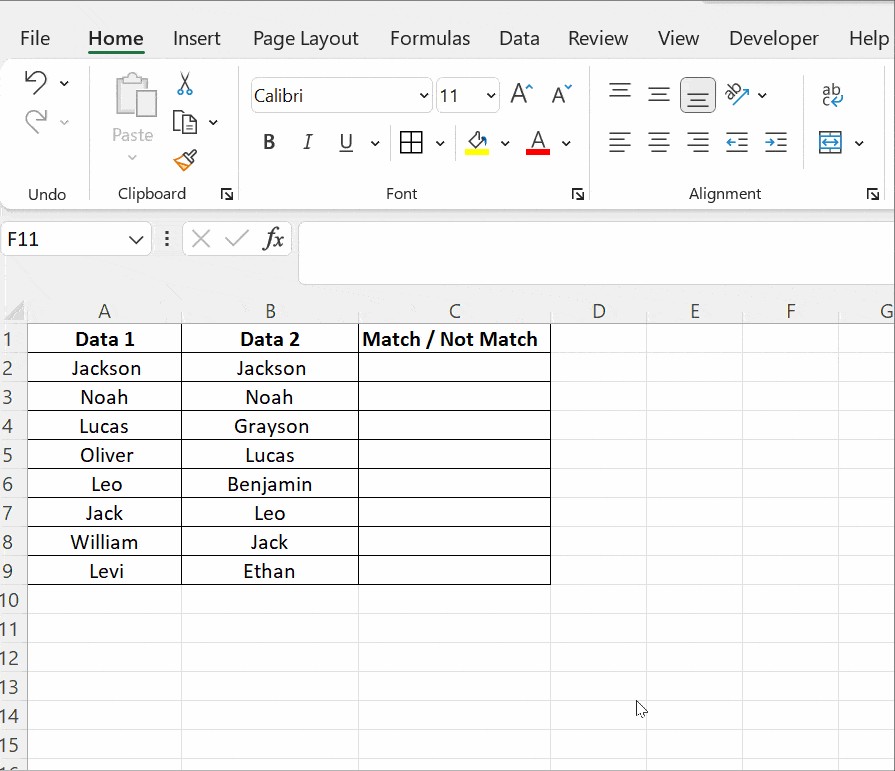
2.1. Comparing Two Columns Using the Equals Operator

You can compare two columns row by row to find matching data by displaying the result as Match or Not Match. Using the formula =A2=B2 in the example below helps find matching data, with the result shown as True or False.

In cell C2, enter the formula and press Enter. Then, drag it down to the end of the table. The formula returns TRUE if the values in the rows being compared are the same, and FALSE if the values are different.

2.2. Comparing Two Columns Using the IF Condition

In Excel, you can compare two columns using the IF condition. The formula to compare two columns is =IF(A2=B2,”Match”,” “). This returns the result as Match against the rows containing matching values, and the remaining rows are left blank.

You can also use the same formula to identify and return mismatching values by showing an additional result when the IF condition is false. The formula is =IF(A2=B2,”Match”,”Not a Match”).

To compare two columns in Excel for differences, replace the equals sign with the non-equality sign (<>). The formula is =IF(A2<>B2,”Match”,”Not a Match”).

2.3. Using the EXACT() Function for Case-Sensitive Comparison

The EXACT() function is useful when comparing two columns in Excel and you need to find values that are case-sensitive.

The EXACT() function compares two text strings and returns TRUE if they are the same and FALSE otherwise. This function is case-sensitive but ignores formatting differences. The syntax is =EXACT(text1, text2), where both text1 and text2 are required arguments.

For example, consider columns data1 and data2 containing two text strings, “Nova Scotia,” in columns A and B.

The formula, =IF(A2=B2, “Match”, “Mismatch”), when applied to cell C2, returns a match because it is case-insensitive.

To make the IF condition case-sensitive, use the formula =IF(EXACT(A2, B2), “Match”, “Mismatch”).

The EXACT() function returns values as true or false. The function works by executing the inner function first, and then the result is returned. In the above example, the EXACT() function returns a false value to the outer function IF.

The general operation of the IF condition is such that if it returns true, the first argument in the function is returned; otherwise, the second argument is returned.

2.4. Conditional Formatting for Highlighting Differences and Similarities

To use conditional formatting, click Home, then Styles, and follow these steps: Conditional Formatting → Highlight Cell Rules → Duplicate Values. A dialogue box will appear. From there, you can choose the values from the drop-down menu.

Apply the formatting condition to the cells. You can choose any conditions: Duplicate or Unique.
Format cells that contain: (options) values with (options)

For example, consider two datasets. The set of names is in columns Data1 and Data2. Not all the names in Data1 are present in Data2. Use Conditional Formatting to find and highlight the data present in both columns.

Before using Conditional Formatting, select the entire table and perform the steps above. Choose Duplicate if you want to find the names in both columns. To highlight them, choose any option: filling with color, changing the text color, or changing the cell border.

The last option is Custom Format. Choose this option if you prefer to highlight the cell with a color of your choice other than the ones specified in the drop-down menu.

Another option is Unique. Use this if you wish to highlight cells containing data that is not repeated. That is, you want to highlight the unique cells.

Instead of selecting Duplicate, choose Unique from the drop-down list and apply any option, such as filling with color, changing the text color, or changing the cell border.

Tip: If you want to clear the formatting you performed on the cells, click Conditional Formatting → Clear Rules → Clear Rules from Selected Cells.

You can use conditional formatting when you don’t want a third column showing the results of comparing the two columns. Here, you can highlight duplicate (matching) and unique (different) data to show which rows have the same data or use an additional column to display values indicating whether the data matches. These methods are more suitable for smaller tables. For large spreadsheets, you may need more complex methods.

2.5. Utilizing Lookup Functions to Compare Two Columns

The LOOKUP function searches for a particular value in a single row or column and returns the corresponding value from another row or column. There are various lookup functions: HLOOKUP, VLOOKUP, and XLOOKUP. H and V stand for horizontal and vertical, respectively, and the XLOOKUP function is a combination of both HLOOKUP and VLOOKUP.

The example below compares two columns in Excel to look for differences using VLOOKUP().

Column A contains the list of exams taken by a student, and column B is the list of subjects the student passed. The result sheet must contain a list of all the subjects. The VLOOKUP() function is applied in cell C2 as =VLOOKUP(A2, $B$2:$B$5,1,0).

Drag the formula to apply it to all cells below C2. You will find the result in column C with the subjects that are cleared and those that have not been cleared as #N/A. The formula in Excel to compare two columns using VLOOKUP is as follows:

VLOOKUP(A2,..,..,..) – takes the value in cell A2.
VLOOKUP(A2, $B$2:$B$5,..,..) – compares with all values in cells from B2 to B5. This is why the cells in the range B2:B5 are locked using an absolute reference. The $ symbol before the cell reference is called an absolute reference.
VLOOKUP(A2, $B$2:$B$5,1,..) – the third argument is the col_index_num, which specifies the position of the column to compare from the lookup value A2. In the above example, the subjects list is in column A, and the column with which it has to compare is 1 column away. Hence, the value 1.
VLOOKUP(A2, $B$2:$B$5,1,0) – this is the last argument that takes a logical value, either 0 or 1. If you wish to find the exact match, mention 0 (zero). If you want VLOOKUP() to return the closest match sorted in ascending order, mention 1 in this argument.

3. Advanced Techniques for Comparing Columns in Excel

For more complex data comparisons, advanced techniques can provide more granular and insightful results.

3.1. Using Array Formulas for Complex Comparisons

Array formulas allow you to perform calculations on multiple values at once, making them useful for complex comparisons.

Syntax: Array formulas are entered by pressing Ctrl + Shift + Enter.
Example: To compare two columns and return an array of matching values, you can use an array formula like: {=IF(A1:A10=B1:B10, “Match”, “Mismatch”)}.
Benefits: Array formulas can handle complex conditions and multiple criteria, providing more detailed comparison results.

3.2. Combining Functions for Enhanced Data Analysis

Combining multiple Excel functions can create powerful formulas for detailed data analysis.

Example: Using the SUMPRODUCT and ISNUMBER functions together can count the number of matching values between two columns.
=SUMPRODUCT(–(ISNUMBER(MATCH(A1:A10, B1:B10, 0))))
Explanation: This formula checks for matching values in columns A and B and returns the count of matches.
Benefits: Combining functions allows for more flexible and customized data analysis, providing insights tailored to specific needs.

3.3. Leveraging Power Query for Data Transformation and Comparison

Power Query is a powerful data transformation and analysis tool built into Excel. It allows you to import, clean, transform, and compare data from multiple sources.

Steps:
1. Import Data: Import the two columns into Power Query.
2. Transform Data: Clean and transform the data as needed.
3. Merge Queries: Merge the two queries based on a common column.
4. Compare Columns: Use custom columns to compare values and identify matches or differences.
Benefits: Power Query can handle large datasets, automate data transformation, and provide advanced data comparison capabilities.

4. Practical Applications of Column Comparison in Excel

Column comparison is useful in many practical scenarios.

4.1. Identifying Duplicate Entries in Large Datasets

Comparing columns can quickly identify duplicate entries in large datasets, ensuring data accuracy and consistency.

Method: Use conditional formatting or the COUNTIF function to highlight or count duplicate entries.
Example: Use conditional formatting to highlight duplicate values in a column containing customer IDs.

4.2. Validating Data Consistency Across Multiple Worksheets

Comparing columns across multiple worksheets can validate data consistency, ensuring that data is synchronized and accurate across different sheets.

Method: Use the VLOOKUP function or Power Query to compare data across worksheets.
Example: Compare customer data in one worksheet with transaction data in another to ensure that all transactions are linked to valid customer records.

4.3. Comparing Product Lists and Inventory Management

Comparing product lists and inventory data can help manage inventory levels, identify discrepancies, and optimize stock management.

Method: Use the VLOOKUP function or conditional formatting to compare product lists and identify missing or mismatched items.
Example: Compare a product list with inventory data to identify items that are out of stock or have incorrect inventory levels.

5. Addressing Common Challenges in Column Comparison

While comparing columns in Excel is a powerful tool, it can come with its own set of challenges.

5.1. Handling Different Data Types

Data types can vary, such as numbers, text, dates, and logical values, which can affect comparison accuracy.

Solution: Use Excel functions to convert data types to a uniform format before comparison.
- TEXT Function: Converts numbers and dates to text. =TEXT(A1, “0”)
- VALUE Function: Converts text to numbers. =VALUE(B1)
- DATE Function: Ensures dates are in the same format. =DATE(YEAR(C1), MONTH(C1), DAY(C1))
Example: If one column contains numbers formatted as text and another contains true numerical values, use the VALUE function to convert the text values to numbers before comparing.

5.2. Dealing with Case Sensitivity

Case sensitivity can lead to mismatches in comparisons if not handled correctly.

Solution: Use functions that ignore case or convert text to a uniform case.
- UPPER Function: Converts text to uppercase. =UPPER(A1)
- LOWER Function: Converts text to lowercase. =LOWER(B1)
- EXACT Function: For case-sensitive comparisons. =EXACT(A1, B1)
Example: If comparing names, use the UPPER or LOWER function to ensure that “John” and “john” are treated as the same.

5.3. Managing Large Datasets

Large datasets can slow down Excel and make comparisons difficult.

Solution: Use efficient methods and tools to manage and compare large datasets.
- Power Query: Designed for handling large datasets and performing complex transformations.
- Array Formulas: Use with caution, as they can be resource-intensive on large datasets.
- Excel Tables: Can improve performance by structuring data and optimizing calculations.
Example: Use Power Query to import and compare two large CSV files, performing transformations and comparisons efficiently.

6. Best Practices for Efficient Column Comparison

Following best practices can help ensure accurate and efficient column comparisons.

6.1. Preparing Data for Comparison

Data preparation is crucial for accurate and reliable comparisons.

Clean Data: Remove or correct errors, inconsistencies, and irrelevant data.
Standardize Data: Ensure data is in a consistent format (e.g., dates, numbers, text).
Remove Duplicates: Eliminate duplicate entries to avoid skewing comparison results.
Trim Spaces: Remove leading and trailing spaces that can cause mismatches.

6.2. Choosing the Right Comparison Method

Selecting the appropriate method is essential for efficiency and accuracy.

Simple Comparisons: Use basic formulas like =A1=B1 or conditional formatting.
Complex Comparisons: Use array formulas, combined functions, or Power Query.
Case-Sensitive Comparisons: Use the EXACT function.
Large Datasets: Use Power Query or Excel Tables.

6.3. Automating the Comparison Process

Automation can save time and reduce the risk of manual errors.

Macros: Use VBA macros to automate repetitive comparison tasks.
Power Query: Automate data import, transformation, and comparison steps.
Dynamic Formulas: Use dynamic formulas that automatically adjust as data changes.

7. Real-World Examples of Column Comparison

Real-world examples illustrate the practical applications of column comparison in various industries.

7.1. Finance: Reconciling Bank Statements

Financial analysts use Excel to reconcile bank statements by comparing transaction records.

Scenario: Comparing a list of transactions in a bank statement with a list of transactions in an accounting system.
Method: Use the VLOOKUP function to match transactions and identify any discrepancies.
Benefits: Ensures accurate financial reporting and identifies potential errors or fraud.

7.2. Healthcare: Validating Patient Records

Healthcare providers use Excel to validate patient records across different systems.

Scenario: Comparing patient data in an electronic health record (EHR) system with data in a billing system.
Method: Use the IF function and conditional formatting to identify mismatches in patient information.
Benefits: Ensures accurate patient data and reduces the risk of billing errors.

7.3. Retail: Analyzing Sales Data

Retailers use Excel to analyze sales data and optimize inventory management.

Scenario: Comparing sales data with inventory data to identify trends and manage stock levels.
Method: Use Power Query to combine and compare data from different sources, and use conditional formatting to highlight key trends.
Benefits: Optimizes inventory levels, reduces stockouts, and improves sales performance.

8. Tips and Tricks for Effective Column Comparison

Effective column comparison involves several tips and tricks to enhance accuracy and efficiency.

8.1. Using Helper Columns

Helper columns can simplify complex comparisons by breaking them down into smaller, more manageable steps.

Scenario: Comparing two columns based on multiple criteria.
Method: Create helper columns to perform intermediate calculations and then combine the results in a final comparison column.
Benefits: Simplifies complex formulas and makes the comparison process easier to understand.

8.2. Using Named Ranges

Named ranges can make formulas easier to read and maintain.

Scenario: Comparing two columns using the VLOOKUP function.
Method: Define named ranges for the lookup range and the comparison column, and then use the named ranges in the VLOOKUP formula.
Benefits: Makes formulas more readable and easier to update.

8.3. Leveraging Keyboard Shortcuts

Keyboard shortcuts can speed up the comparison process.

Ctrl + Space: Selects an entire column.
Shift + Space: Selects an entire row.
Ctrl + D: Fills down a formula to the selected cells.
Ctrl + R: Fills right a formula to the selected cells.

9. Frequently Asked Questions

9.1. How can I compare two columns in Excel to find matching data?

You can compare two columns in Excel to find matching data by using the =A2=B2 formula, which returns TRUE if the values match and FALSE otherwise. Alternatively, you can use the IF function to display “Match” or “Not Match” based on whether the values are the same.

9.2. How do I compare two columns for differences in Excel?

To compare two columns for differences, use the formula =IF(A2<>B2, “Different”, “Same”). This formula checks if the values in the two cells are not equal and returns “Different” if they are, and “Same” if they are equal.

9.3. Can I perform a case-sensitive comparison in Excel?

Yes, you can perform a case-sensitive comparison in Excel using the EXACT function. The formula =IF(EXACT(A2, B2), “Match”, “Mismatch”) will return “Match” only if the values are exactly the same, including case.

9.4. How can I highlight matching or unique values in two columns?

You can use conditional formatting to highlight matching or unique values in two columns. Select the columns, go to Home → Conditional Formatting → Highlight Cells Rules, and choose either Duplicate Values or Unique Values.

9.5. What is the best way to compare two columns with large datasets?

For large datasets, using Power Query is an efficient method. Import the data into Power Query, merge the columns based on a common identifier, and then compare the values using a custom column.

9.6. How do I use VLOOKUP to compare two columns?

You can use VLOOKUP to check if values from one column exist in another. For example, =VLOOKUP(A2, $B$2:$B$10, 1, FALSE) will look for the value in A2 within the range B2:B10. If found, it returns the matching value from column B; otherwise, it returns #N/A.

9.7. How can I compare two columns across different Excel sheets?

To compare two columns across different sheets, reference the columns using the sheet name in your formula. For example, =IF(Sheet1!A2=Sheet2!B2, “Match”, “Mismatch”) compares the value in cell A2 of Sheet1 with the value in cell B2 of Sheet2.

9.8. Can I count the number of matches between two columns in Excel?

Yes, you can count the number of matches using the SUMPRODUCT and IF functions. For example, =SUMPRODUCT(–(A1:A10=B1:B10)) will return the number of rows where the values in columns A and B match.

9.9. What are helper columns and how do they help in column comparison?

Helper columns are additional columns used to simplify complex comparisons by breaking them down into smaller, more manageable steps. They allow you to perform intermediate calculations and then combine the results in a final comparison column.

9.10. How can I automate the column comparison process in Excel?

You can automate the column comparison process using VBA macros or Power Query. VBA macros can be used to write custom comparison routines, while Power Query can automate data import, transformation, and comparison steps.

10. Conclusion: Mastering Column Comparison in Excel

In conclusion, mastering the art of comparing columns in Excel is a crucial skill for anyone working with data. The techniques outlined in this guide, from basic formulas to advanced functions like Power Query, provide a comprehensive toolkit for efficiently and accurately comparing data. Whether you are identifying discrepancies, validating data, or analyzing trends, these methods will enhance your productivity and decision-making capabilities.

By understanding and applying these strategies, you can unlock valuable insights and improve the overall quality of your data analysis. Remember to explore and experiment with these techniques to find the methods that best suit your specific needs and datasets.

If you’re looking for more ways to enhance your data analysis skills and gain deeper insights from your data, visit COMPARE.EDU.VN. We offer a wide range of resources, including detailed tutorials and expert advice, to help you make informed decisions and stay ahead in today’s data-driven world.

Ready to elevate your Excel skills and make data-driven decisions with confidence? Visit COMPARE.EDU.VN today and discover how our resources can empower you to compare, analyze, and conquer your data challenges!

Address: 333 Comparison Plaza, Choice City, CA 90210, United States

WhatsApp: +1 (626) 555-9090

Website: compare.edu.vn