Comparing two columns in Excel can be efficiently done using various methods like conditional formatting, formulas, and lookup functions, enabling you to highlight differences or find matches. At COMPARE.EDU.VN, we provide detailed comparisons and guides to help you master these techniques. Understanding these methods is crucial for data analysis and decision-making, enabling you to identify unique or duplicate values, compare data row by row, and leverage lookup formulas for in-depth analysis. Explore different comparison techniques, data validation and spreadsheet analysis on COMPARE.EDU.VN
1. Why Is Comparing Two Columns in Excel Important?
Comparing two columns in Excel is important for data analysis and decision-making. It helps data analysts determine whether a cell contains data, identify missing or duplicate information, and make informed decisions based on data.
Excel spreadsheets are versatile tools for data storage, manipulation, and decision-making. Comparing two columns allows data analysts to:
- Identify whether cells contain data.
- Spot missing or duplicate information.
- Make informed decisions based on the data.
- Streamline the data comparison process, saving time and reducing errors compared to manual methods.
2. What Are the Common Methods to Compare Two Columns in Excel?
Several methods are available for comparing two columns in Excel, including:
- Highlighting unique or duplicate values using functions.
- Displaying unique or duplicate cells using conditional formatting or formulas.
- Performing a row-by-row comparison.
- Using LOOKUP formulas.
These methods cater to different comparison needs, allowing users to identify discrepancies, find matches, and perform detailed data analysis.
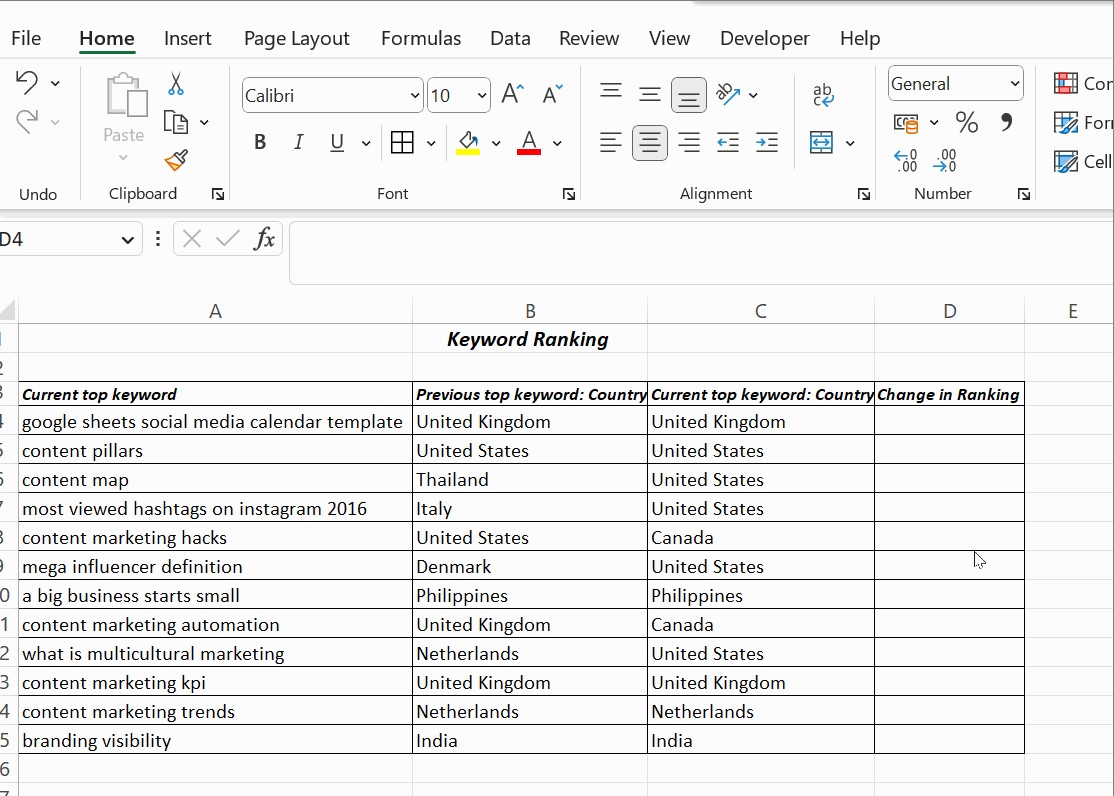
3. How Do You Compare Two Columns Using the Equals Operator?
You can compare two columns row by row and find matching data by using the equals operator (=). The formula =column1=column2 returns TRUE if there’s a match or FALSE if the values differ.
Example:
- In cell D4, enter the formula
=B4=C4and press Enter. - Drag the formula down to the end of the table.
The formula returns TRUE if the values in columns B and C match in that row, and FALSE if they don’t.
This method is straightforward and provides a quick way to identify exact matches between two columns.
4. How Can You Compare Two Columns Using the IF Condition?
You can use the IF condition to compare two columns in Excel. The formula =IF(B4=C4, "Yes", " ") returns “Yes” for matching values and leaves the cell blank for non-matching values. To identify mismatching values, use =IF(B4=C4, "Yes", "No").
Example:
- In cell D4, enter the formula
=IF(B4=C4, "Yes", " ")and press Enter. - Drag the formula down to the end of the table.
This will display “Yes” in column D for rows where the values in columns B and C match, and leave the cell blank where they don’t.
To compare two columns for differences, replace the equals sign with the non-equality sign (<>). The formula =IF(A2<>B2, "Match", "Not a Match") returns “Match” if the values are different and “Not a Match” if they are the same.
5. What Is the EXACT() Function and How Does It Enhance Column Comparison?
The EXACT() function compares two text strings and returns TRUE only if they are identical, including capitalization. The syntax is =EXACT(text1, text2). This function is case-sensitive and ignores formatting differences.
Example:
To perform a case-sensitive comparison, use the formula =IF(EXACT(B4, C4), "Match", "Mismatched").
This formula returns “Match” only if the text in B4 and C4 is identical, including capitalization. Otherwise, it returns “Mismatched”.
The EXACT() function enhances column comparison by ensuring that the comparison is case-sensitive, which is essential when the case of the text matters.
6. How Can Conditional Formatting Be Used to Compare Two Columns?
Conditional formatting can be used to highlight duplicate or unique values in two columns without needing a third column for results.
Steps:
- Select the columns you want to compare.
- Click Home, then Conditional Formatting.
- Choose Highlight Cell Rules and then Duplicate Values.
- In the dialog box, select Duplicate or Unique from the drop-down menu.
- Choose a formatting option (e.g., fill color, text color, cell border).
- Click OK.
Example:
To highlight values that appear in both columns, choose Duplicate. To highlight values that are unique to each column, choose Unique.
To clear formatting, click Conditional Formatting → Clear Rules → Clear Rules from Selected Cells.
Conditional formatting is useful when you want a visual representation of matching or differing data without adding extra columns.
7. How Do LOOKUP Functions Aid in Comparing Two Columns?
LOOKUP functions, such as VLOOKUP, HLOOKUP, and XLOOKUP, search for a value in a row or column and return a corresponding value from another row or column.
Example using VLOOKUP:
Suppose Column A contains a list of keywords, and Column B contains parent keywords. To find the matching parent keywords for each keyword in Column A:
- In cell C4, enter the formula
=VLOOKUP(A4, $B$4:$B$15, 1, 0). - Drag the cell to apply the formula to all cells below C4.
The formula in detail:
VLOOKUP(A4, ...): This takes the value in cell A4 (the keyword).VLOOKUP(A4, $B$4:$B$15, ...): This compares the value in A4 to the values in cells B4 to B15 (the parent keywords). The$symbol creates an absolute reference, ensuring the range B4:B15 doesn’t change when you drag the formula.VLOOKUP(A4, $B$4:$B$15, 1, ...): The third argument,1, specifies the column index number, which is the position of the column to compare from the lookup value A4.VLOOKUP(A4, $B$4:$B$15, 1, 0): The last argument,0, specifies that you want to find an exact match.
The result in Column C will show the matching parent keyword for each keyword in Column A. If no match is found, it will return an error (#N/A).
8. Can You Explain VLOOKUP’s Role in Identifying Differences Between Columns?
VLOOKUP (Vertical Lookup) searches for a value in the first column of a range and returns a value from a specified column in the same row. It is useful for identifying differences between columns by finding matches and highlighting discrepancies.
How it works:
- Lookup Value: The value you want to find in the first column of a range.
- Table Array: The range of cells where the lookup value is searched.
- Col Index Num: The column number in the table array from which the matching value is returned.
- Range Lookup: A logical value that specifies whether to find an exact match (FALSE) or an approximate match (TRUE).
Example:
Suppose you have two columns, A and B, and you want to see if the values in column A exist in column B. You can use the following formula in column C:
=VLOOKUP(A1,B:B,1,FALSE)
- A1: The lookup value (the value from column A).
- B:B: The table array (column B).
- 1: The column index number (since we are looking in column B, which is the first and only column in our table array).
- FALSE: Specifies that we want an exact match.
If the value in A1 is found in column B, the formula will return that value. If not found, it returns #N/A, indicating a difference.
9. What Is the Formula to Compare Three or More Columns in Excel?
To compare three or more columns in Excel, you can use the IF() function combined with the AND() or OR() functions.
To find matches in all cells across multiple columns:
Use the formula =IF(AND(A2=B2, A2=C2), "Full match", ""). This formula returns “Full match” if all values in columns A, B, and C are the same in a given row, and an empty string if they are not.
To find matches in any two cells in the same row:
Use the formula =IF(OR(A2=B2, B2=C2, A2=C2), "Match", ""). This formula returns “Match” if any two values in columns A, B, and C are the same in a given row, and an empty string if none match.
Example:
| Column A | Column B | Column C | Result (Full match) | Result (Any Match) |
|---|---|---|---|---|
| 1 | 1 | 1 | Full match | Match |
| 1 | 2 | 1 | Match | |
| 1 | 2 | 3 |


These formulas can be extended to compare any number of columns by adding more conditions to the AND() or OR() functions.
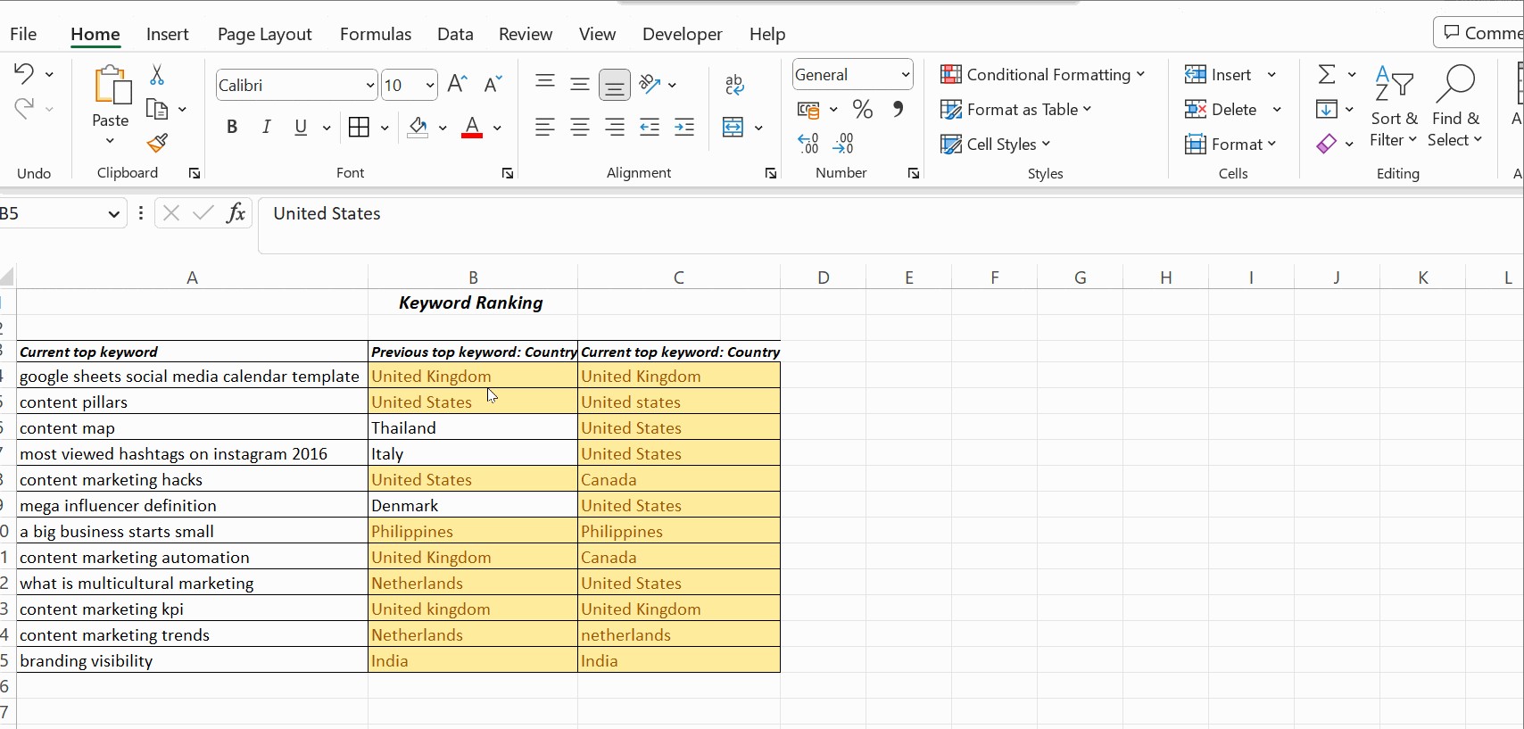
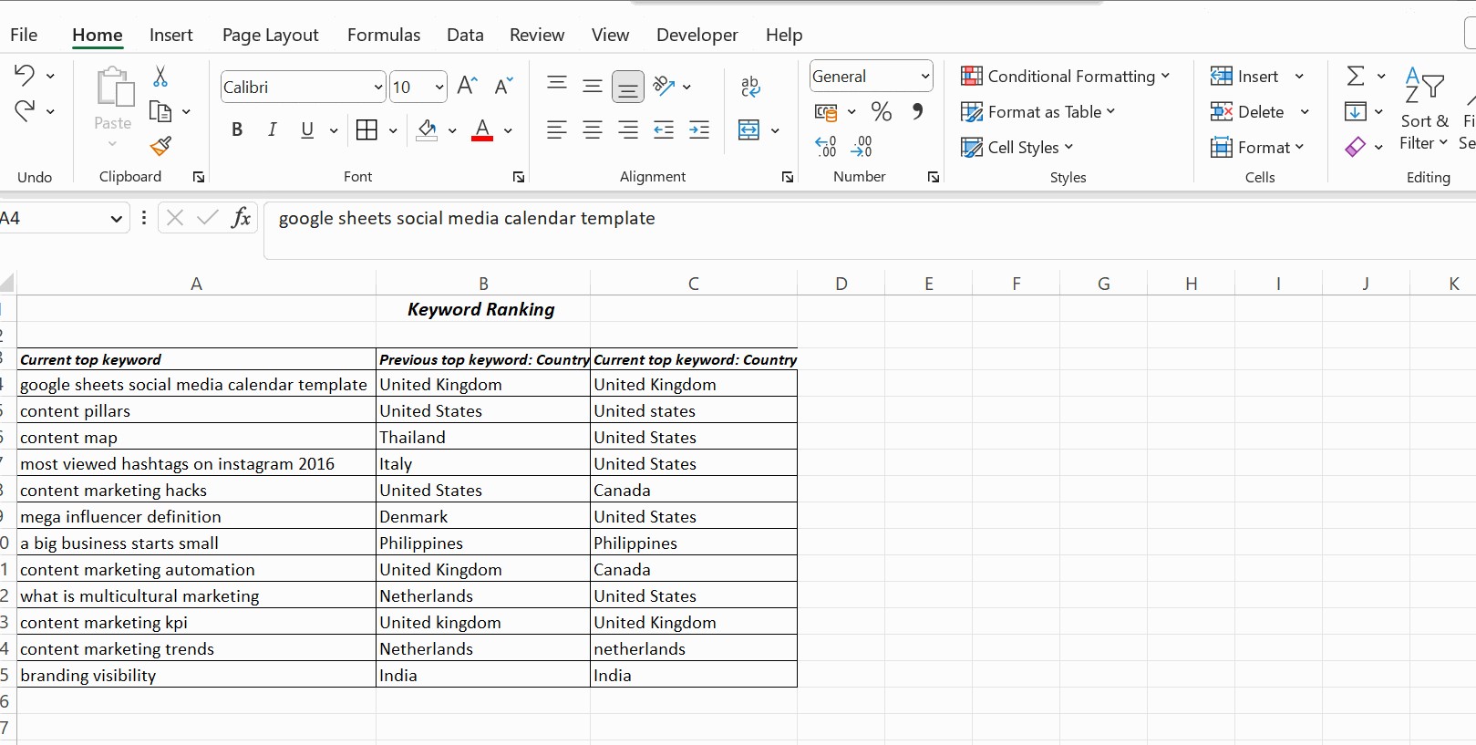
10. How Can You Identify Row Differences Without Formulas in Excel?
To identify row differences without using formulas, you can use the “Go To Special” feature in Excel.
Steps:
- Select both columns of data.
- Go to Home → Find & Select → Go To Special.
- Choose Row Differences and click OK.
Excel will highlight the cells that are different in each row. Matching cells will appear white, while unmatched cells will be gray.
This method is quick and provides a visual way to identify differences without the need for formulas.
11. What Are Some Advanced Techniques for Comparing Columns in Excel?
Advanced techniques for comparing columns in Excel include using array formulas, combining multiple functions, and using VBA (Visual Basic for Applications) for more complex comparisons.
Array Formulas
Array formulas can perform calculations on entire ranges of cells. For example, to compare two columns and return an array of TRUE/FALSE values:
- Select a range of cells where you want the results to appear.
- Enter the formula
=A1:A5=B1:B5. - Press
Ctrl + Shift + Enterto enter the formula as an array formula.
This will compare each cell in the range A1:A5 with the corresponding cell in the range B1:B5 and return an array of TRUE/FALSE values.
Combining Multiple Functions
You can combine multiple functions to perform more complex comparisons. For example, to check if two columns have the same values regardless of their order:
=IF(SUMPRODUCT(--(COUNTIF(A1:A5,B1:B5)>0))=ROWS(A1:A5), "Same Values", "Different Values")
This formula checks if all values in column B exist in column A, regardless of their order.
Using VBA
For more complex comparisons, you can use VBA to write custom functions. For example, to compare two columns and highlight differences:
Sub CompareColumns()
    Dim i As Long
    Dim lastRow As Long

    lastRow = Cells(Rows.Count, "A").End(xlUp).Row

    For i = 1 To lastRow
        If Cells(i, "A").Value <> Cells(i, "B").Value Then
            Cells(i, "A").Interior.Color = vbYellow
            Cells(i, "B").Interior.Color = vbYellow
        End If
    Next i
End Sub
This VBA code compares column A and column B and highlights the cells that are different in yellow.
12. How Can COMPARE.EDU.VN Assist in Mastering Excel Column Comparisons?
COMPARE.EDU.VN offers detailed guides and comparisons to help users master Excel column comparisons. We provide step-by-step instructions, examples, and advanced techniques to efficiently compare data and make informed decisions.
Our resources include:
- Detailed articles on various Excel functions and formulas.
- Comparative analyses of different comparison methods.
- Tips and tricks for optimizing data analysis.
By using compare.edu.vn, users can enhance their Excel skills and streamline their data comparison processes.
13. What Are Common Mistakes to Avoid When Comparing Columns in Excel?
When comparing columns in Excel, several common mistakes can lead to inaccurate results. Here are some pitfalls to avoid:
-
Ignoring Case Sensitivity:
- Mistake: Not considering that Excel functions like
IFand simple=comparisons are not case-sensitive. - Solution: Use the
EXACT()function for case-sensitive comparisons.
- Mistake: Not considering that Excel functions like
-
Overlooking Trailing Spaces:
- Mistake: Failing to trim extra spaces at the beginning or end of cells.
- Solution: Use the
TRIM()function to remove extra spaces before comparing.
-
Incorrect Range References:
- Mistake: Using incorrect cell ranges in formulas, leading to missed or incorrect comparisons.
- Solution: Double-check and ensure that all range references in formulas are accurate.
-
Forgetting Absolute vs. Relative References:
- Mistake: Not using absolute references (
$) when you need to keep a cell reference constant while dragging formulas. - Solution: Use absolute references where necessary to prevent formulas from changing incorrectly.
- Mistake: Not using absolute references (
-
Misunderstanding Data Types:
- Mistake: Comparing different data types (e.g., numbers as text).
- Solution: Ensure that the data types being compared are consistent, using functions like
VALUE()to convert text to numbers if needed.
-
Ignoring Errors:
- Mistake: Not handling potential errors (e.g.,
#N/AfromVLOOKUP) in formulas. - Solution: Use
IFERROR()to handle errors and provide meaningful results.
- Mistake: Not handling potential errors (e.g.,
-
Overcomplicating Formulas:
- Mistake: Creating unnecessarily complex formulas that are hard to understand and debug.
- Solution: Keep formulas as simple as possible and break down complex tasks into smaller, manageable steps.
-
Not Clearing Conditional Formatting:
- Mistake: Applying multiple conditional formatting rules without clearing previous ones, leading to unexpected results.
- Solution: Clear existing rules before applying new ones to avoid conflicts.
-
Failing to Test Thoroughly:
- Mistake: Not testing formulas and comparisons with various scenarios to ensure accuracy.
- Solution: Test with different data sets and edge cases to validate the results.
-
Misusing Wildcards:
- Mistake: Using wildcards (
*,?) incorrectly in functions likeCOUNTIForSUMIF. - Solution: Understand how wildcards work and use them appropriately for partial matches.
- Mistake: Using wildcards (
By avoiding these common mistakes, you can improve the accuracy and reliability of your column comparisons in Excel.
14. How Do Data Validation Techniques Enhance Column Comparison Accuracy?
Data validation techniques enhance column comparison accuracy by ensuring data consistency and integrity. By setting rules for what data can be entered into a cell, you reduce the risk of errors and inconsistencies that can complicate comparisons.
Key benefits of using data validation:
-
Ensuring Consistent Data Types:
- Data validation can enforce specific data types (e.g., numbers, dates, text) in columns, preventing type-related comparison errors.
- Example: Restricting a column to accept only numerical values ensures that comparisons with another numerical column are accurate.
-
Limiting Input to Predefined Lists:
- Using dropdown lists for data entry ensures that only predefined, standardized values are entered, reducing variations and typos.
- Example: A column for “Country” can be restricted to a list of valid country names, ensuring consistency in comparisons.
-
Setting Length and Format Restrictions:
- Data validation can enforce length limits and specific formats (e.g., email addresses, phone numbers), ensuring uniformity.
- Example: Limiting the number of characters in a product code column ensures that all entries adhere to a specific format.
-
Preventing Duplicate Entries:
- Data validation can be used to prevent duplicate entries within a column, ensuring that comparisons focus on unique values.
- Example: Preventing duplicate customer IDs in a customer database ensures accurate comparisons with other data sets.
-
Providing Input Messages and Error Alerts:
- Custom input messages guide users on the expected data format, while error alerts notify them of invalid entries, reducing mistakes.
- Example: An input message can specify the required format for a date field, and an error alert can prevent the entry of invalid dates.
-
Improving Data Cleaning Processes:
- Data validation highlights inconsistencies and errors, making it easier to clean and standardize data before comparison.
- Example: Identifying and correcting invalid entries in a zip code column before comparing it with another address database.
-
Enhancing Data Integrity:
- By enforcing data rules, validation ensures that the data remains reliable and trustworthy, which is crucial for accurate comparisons and analysis.
- Example: Ensuring that all entries in a sales data column are positive numbers prevents skewed comparisons and inaccurate reports.
-
Streamlining Data Entry:
- Consistent data entry reduces the need for extensive data cleaning, saving time and effort in preparing data for comparisons.
- Example: Standardizing date formats across different columns simplifies the process of comparing date-related data.
By implementing data validation, you can significantly improve the quality and consistency of your data, leading to more accurate and reliable column comparisons in Excel.
15. Can You Provide Scenarios Where Comparing Columns in Excel Is Crucial?
Comparing columns in Excel is crucial in various scenarios across different industries and functions. Here are some examples:
-
Finance and Accounting:
- Scenario: Reconciling bank statements with internal records to identify discrepancies and ensure accurate financial reporting.
- Use Case: Comparing transaction amounts and dates in two columns to find missing or incorrect entries.
-
Sales and Marketing:
- Scenario: Analyzing customer data from different sources (e.g., CRM, marketing automation tools) to identify duplicate leads and ensure consistent customer information.
- Use Case: Comparing email addresses or phone numbers in two columns to merge duplicate customer profiles.
-
Human Resources:
- Scenario: Comparing employee data across different HR systems (e.g., payroll, benefits) to ensure data consistency and identify discrepancies.
- Use Case: Comparing employee IDs or names in two columns to update employee records accurately.
-
Inventory Management:
- Scenario: Comparing inventory levels in different warehouses to optimize stock distribution and prevent stockouts or overstocking.
- Use Case: Comparing product codes and quantities in two columns to identify discrepancies in inventory counts.
-
Project Management:
- Scenario: Comparing planned vs. actual project timelines to track progress and identify delays.
- Use Case: Comparing task start and end dates in two columns to monitor project milestones.
-
Data Analysis:
- Scenario: Validating data integrity by comparing data from different sources to identify errors or inconsistencies.
- Use Case: Comparing customer data with demographic data to identify target market segments.
-
Quality Control:
- Scenario: Comparing product specifications with actual measurements to identify defects and ensure compliance with quality standards.
- Use Case: Comparing dimensions or weights in two columns to detect manufacturing errors.
-
Customer Support:
- Scenario: Analyzing customer feedback data from different channels to identify common issues and improve service quality.
- Use Case: Comparing customer complaint topics in two columns to identify recurring problems.
-
Supply Chain Management:
- Scenario: Comparing purchase orders with invoices to verify accuracy and prevent payment errors.
- Use Case: Comparing product prices and quantities in two columns to ensure correct billing.
-
Research and Development:
- Scenario: Comparing experimental results from different trials to identify significant findings.
- Use Case: Comparing data points in two columns to validate research hypotheses.
In each of these scenarios, comparing columns in Excel helps ensure data accuracy, consistency, and reliability, leading to better decision-making and improved operational efficiency.
16. How Can You Automate Column Comparisons in Excel Using VBA?
Automating column comparisons in Excel using VBA (Visual Basic for Applications) can significantly streamline repetitive tasks. Here’s how you can do it:
-
Open the VBA Editor:
- Press
Alt + F11to open the VBA editor in Excel.
- Press
-
Insert a New Module:
- In the VBA editor, go to
Insert>Module.
- In the VBA editor, go to
-
Write the VBA Code:
- Here’s an example VBA code to compare two columns (A and B) and highlight the differences in column C:
Sub CompareColumns()
    Dim ws As Worksheet
    Dim lastRow As Long
    Dim i As Long

    ' Set the worksheet
    Set ws = ThisWorkbook.Sheets("Sheet1") ' Replace "Sheet1" with your sheet name

    ' Find the last row with data in column A
    lastRow = ws.Cells(ws.Rows.Count, "A").End(xlUp).Row

    ' Loop through each row
    For i = 2 To lastRow ' Assuming data starts from row 2
        ' Compare values in column A and column B
        If ws.Cells(i, "A").Value <> ws.Cells(i, "B").Value Then
            ' Write "Different" in column C if values are not the same
            ws.Cells(i, "C").Value = "Different"
        Else
            ' Write "Same" in column C if values are the same
            ws.Cells(i, "C").Value = "Same"
        End If
    Next i

    ' Optional: Auto-fit column C for better readability
    ws.Columns("C").AutoFit

    MsgBox "Comparison complete!", vbInformation
End Sub-
Explanation of the Code:
Sub CompareColumns(): Starts the subroutine.Dim ws As Worksheet: Declares a worksheet variable.Dim lastRow As Long: Declares a variable to store the last row number.Dim i As Long: Declares a loop counter variable.Set ws = ThisWorkbook.Sheets("Sheet1"): Sets the worksheet to the specified sheet name.lastRow = ws.Cells(ws.Rows.Count, "A").End(xlUp).Row: Finds the last row with data in column A.For i = 2 To lastRow: Loops through each row from row 2 to the last row.If ws.Cells(i, "A").Value <> ws.Cells(i, "B").Value Then: Compares the values in column A and column B.ws.Cells(i, "C").Value = "Different": Writes “Different” in column C if values are not the same.Else: If the values are the same.ws.Cells(i, "C").Value = "Same": Writes “Same” in column C if values are the same.Next i: Moves to the next row.ws.Columns("C").AutoFit: Auto-fits the width of column C for better readability.MsgBox "Comparison complete!", vbInformation: Shows a message box indicating that the comparison is complete.
-
Run the VBA Code:
- Go back to your Excel sheet.
- Press
Alt + F8to open the “Macro” dialog box. - Select
CompareColumnsfrom the list and clickRun.
-
Customize the Code (Optional):
- Change Worksheet: Modify
Sheets("Sheet1")to match your sheet name. - Adjust Columns: Change
"A","B", and"C"to the columns you want to compare and output the results. - Modify Comparison Criteria: Adjust the
Ifstatement to perform different types of comparisons (e.g., case-sensitive comparisons usingStrComp). - Highlight Differences: Instead of writing “Different”, you can change the background color of the cells to highlight differences.
- Change Worksheet: Modify
Here’s an example of how to highlight differences:
ws.Cells(i, "A").Interior.Color = vbYellow
ws.Cells(i, "B").Interior.Color = vbYellow
This code will change the background color of the cells in columns A and B to yellow if they are different.
By automating column comparisons with VBA, you can save time and ensure consistent results, especially when dealing with large datasets.
17. What Are the Best Practices for Optimizing Excel Performance When Comparing Large Datasets?
When comparing large datasets in Excel, optimizing performance is crucial to avoid slow processing and potential crashes. Here are some best practices to enhance Excel’s performance:
-
Use Efficient Formulas:
- Avoid Volatile Functions: Functions like
NOW()andRAND()recalculate with every change, slowing down performance. Use them sparingly. - Use Indexed Lookups: Prefer
INDEX(MATCH())overVLOOKUP()orHLOOKUP(), as they are generally faster, especially when looking up values in large datasets. - Array Formulas: Use array formulas carefully, as they can be resource-intensive. Try to avoid them if possible, or use helper columns with regular formulas instead.
- Avoid Volatile Functions: Functions like
-
Optimize Data Structure:
- Use Tables: Convert your data ranges to Excel Tables. Tables are optimized for data management and can improve performance with structured references.
- Minimize Unnecessary Data: Remove any unused columns, rows, or sheets. Smaller file sizes lead to better performance.
- Data Types: Ensure consistent data types in columns. Mixed data types can slow down calculations.
-
Disable Automatic Calculations:
- Manual Calculation Mode: Switch to manual calculation mode (
Formulas > Calculation Options > Manual). This prevents Excel from recalculating formulas with every change. Remember to manually calculate when needed by pressingF9.
- Manual Calculation Mode: Switch to manual calculation mode (
-
Use Helper Columns:
- Break Down Complex Formulas: Instead of using one complex formula, break it down into smaller, simpler formulas in helper columns. This can improve calculation speed.
-
Conditional Formatting:
- Limit Conditional Formatting: Too many conditional formatting rules can significantly slow down Excel. Use them sparingly and ensure they are applied only to necessary ranges.
- Optimize Rules: Use formulas that minimize calculations within conditional formatting rules.
-
VBA Optimization:
- Disable Screen Updating: When using VBA, disable screen updating at the beginning of your code and re-enable it at the end. This prevents Excel from redrawing the screen with every change, speeding up the process.
Application.ScreenUpdating = False
' Your code here
Application.ScreenUpdating = True- Turn Off Events: Disable events at the beginning of your VBA code and re-enable them at the end to prevent event-triggered code from running unnecessarily.
Application.EnableEvents = False
' Your code here
Application.EnableEvents = True- Use Efficient Looping: When looping through large datasets, use efficient methods like array manipulation instead of looping through each cell individually.
-
File Management:
- Save as .xlsx or .xlsb: Save your files in the
.xlsx(Excel Workbook) or.xlsb(Excel Binary Workbook) format..xlsbis often faster and more compact. - Avoid Overlinking: Reduce the number of links to external workbooks, as these can slow down performance.
- Save as .xlsx or .xlsb: Save your files in the
-
Hardware Considerations:
- Sufficient RAM: Ensure your computer has enough RAM to handle large datasets.
- Fast Processor: A faster processor can significantly improve calculation speeds.
-
Filter Instead of Copying:
- Use Filters: Instead of copying large amounts of data, use filters to display only the relevant information.
-
Remove Circular References:
- Avoid Circular References: Circular references (where a formula refers back to its own cell, directly or indirectly) can cause Excel to recalculate endlessly. Identify and remove these.
By implementing these best practices, you can significantly improve Excel’s performance when working with large datasets, making your comparisons and analyses more efficient and less prone to errors.
18. How Can I Troubleshoot Common Errors When Comparing Columns In Excel?
Troubleshooting common errors when comparing columns in Excel involves systematically identifying and resolving issues that prevent accurate comparisons. Here’s a breakdown of common errors and how to address them:
-
#N/A Error (VLOOKUP, HLOOKUP, MATCH):
- Cause: The lookup value is not found in the lookup range.
- Troubleshooting Steps:
- Verify that the lookup value exists in the lookup range.
- Check for spelling errors or extra spaces in the lookup value or lookup range.
- Ensure that the data types of the lookup value and the values in the lookup range match.
- Use
IFERROR()to handle the error and provide a meaningful result:=IFERROR(VLOOKUP(A1,B:C,2,FALSE), "Not Found").
-
#VALUE! Error:
- Cause: Incorrect data type or syntax in the formula.
- Troubleshooting Steps:
- Ensure that all cell references are correct and refer to valid ranges.
- Verify that the formula uses the correct operators and functions for the data types being compared.
- Check for text values where numeric values are expected, or vice versa. Use
ISNUMBER()orISTEXT()to check data types.
-
#REF! Error:
- Cause: Invalid cell reference (e.g., deleting a column or row that is referenced in a formula).
- Troubleshooting Steps:
- Review the formula and update any invalid cell references.
- If the referenced cell has been deleted, consider using a different cell or range.
-
Incorrect Results with Conditional Formatting:
- Cause: Incorrectly configured conditional formatting rules.
- Troubleshooting Steps:
- Review the conditional formatting rules to ensure they are applied to the correct range and use the correct criteria.
- Check the order of rules, as the first rule that evaluates to TRUE will be applied.
- Use the “Manage Rules” option to edit or delete conflicting rules.
-
Case Sensitivity Issues:
- Cause: Formulas like
IFand simple comparisons are not case-sensitive, leading to incorrect matches. - Troubleshooting Steps:
- Use the
EXACT()function for case-sensitive comparisons:=IF(EXACT(A1,B1), "Match", "No Match").
- Use the
- Cause: Formulas like
-
Extra Spaces:
- Cause: Extra spaces at the beginning or end of text values can cause comparisons to fail.
- Troubleshooting Steps:
- Use the
TRIM()function to remove extra spaces:=TRIM(A1). - Apply
TRIM()to both columns before comparing:=IF(TRIM(A1)=TRIM(B1), "Match", "No Match").
- Use the
-
Data Type Mismatches:
- Cause: Comparing different data types (e.g., numbers formatted as text).
- Troubleshooting Steps:
- Ensure that the data types being compared are consistent.
- Use
VALUE()to convert text to numbers:=VALUE(A1). - Use
TEXT()to format numbers as text:=TEXT(A1, "0").
-
Circular References:
- Cause: A formula refers back to its own cell, directly or indirectly, causing endless recalculations and potentially incorrect results.
- Troubleshooting Steps:
- Go to
Formulas > Error Checking > Circular Referencesto identify and resolve circular references. - Review the formulas in the identified cells and break the circular dependency.
- Go to
-
Incorrect Range References:
- Cause: Formulas using incorrect cell ranges, leading to missed or incorrect comparisons.
- Troubleshooting Steps:
- Double-check and ensure that all range references in formulas are accurate.
- Use named ranges to make formulas more readable and less prone to errors.
-
Manual Calculation Mode:
- Cause: Excel is in manual calculation mode, preventing formulas from updating automatically.
- Troubleshooting Steps:
- Switch to automatic calculation mode:
Formulas > Calculation Options > Automatic.
- Switch to automatic calculation mode:
By systematically checking for these common errors and applying the appropriate troubleshooting steps, you can ensure accurate and reliable column comparisons in Excel.
19. What Free Online Resources Can Help Me Learn More About Comparing Columns in Excel?
There are many free online resources available to help you learn more about comparing columns in Excel. Here are some of the best options:
-
Microsoft Office Support:
- Website: Microsoft Support
- Content: Microsoft provides comprehensive documentation and tutorials on Excel features, including formulas and functions for comparing columns.
- Benefit: Direct, official information from