How To Compare 2 Tabs In Excel: A Comprehensive Guide

Comparing two tabs in Excel is essential for data validation, identifying discrepancies, and merging information. COMPARE.EDU.VN offers a detailed guide on how to effectively compare two tabs in Excel, ensuring accuracy and efficiency in your data management tasks. This guide provides solutions for everyone from students to professionals.

1. What Are The Best Methods On How To Compare Two Excel Tabs Simultaneously?

Excel offers several methods to compare two tabs simultaneously, catering to different needs and levels of detail required. Here are some effective techniques:

1.1 Viewing Tabs Side By Side

This method is best for visual comparison and is suitable for smaller datasets where you can easily spot differences with your eyes.

1.1.1. Comparing Two Excel Workbooks

If the tabs you want to compare are in different workbooks, follow these steps:

Open Both Workbooks: Open the two Excel files you want to compare.
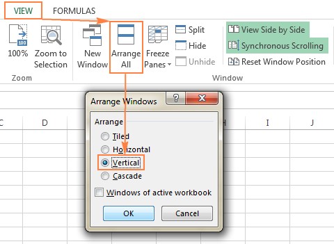
View Side by Side: Go to the View tab, in the Window group, click the View Side by Side button. Excel will arrange the two workbooks horizontally.
Arrange Vertically (Optional): To view the windows vertically, click the Arrange All button (also in the Window group) and select Vertical.
Synchronous Scrolling: Ensure the Synchronous Scrolling option is enabled (located under the View Side by Side button) to scroll through both worksheets simultaneously.

1.1.2. Comparing Two Sheets In The Same Workbook

When the sheets you want to compare are in the same workbook:

Open the Excel File: Open the Excel file containing the two sheets.
New Window: Go to the View tab, in the Window group, and click the New Window button. This opens another window of the same Excel file.
View Side by Side: Enable View Side by Side mode.
Select Sheets: In each window, select the sheet you want to compare.

1.2. Using Excel Formulas

This method is useful for creating a difference report that highlights discrepancies in values.

1.2.1. Creating A Difference Report

Open A New Sheet: Open a new, empty sheet in your Excel workbook.
Enter The Formula: In cell A1 of the new sheet, enter the following formula:
=IF(Sheet1!A1<>Sheet2!A1, "Sheet1:"&Sheet1!A1&" vs Sheet2:"&Sheet2!A1, "")
Copy The Formula: Copy the formula down and to the right by dragging the fill handle (the small square at the bottom right of the cell).
Analyze The Report: The formula compares corresponding cells in Sheet1 and Sheet2. If the values are different, it displays the values from both sheets in the new sheet.

1.3. Conditional Formatting

Conditional formatting can highlight cells with different values directly in the worksheet.

1.3.1. Highlighting Differences With Color

Select All Used Cells: In the worksheet where you want to highlight differences, select all used cells by clicking the upper left cell (usually A1) and pressing Ctrl + Shift + End.
Conditional Formatting Rule:
- Go to the Home tab, in the Styles group, click Conditional Formatting > New Rule.
- Select “Use a formula to determine which cells to format.”
- Enter the following formula: =A1<>Sheet2!A1 (replace “Sheet2” with the name of the other sheet).
- Click the Format button to choose a highlight color.
Apply The Rule: Click OK to apply the rule. Cells with different values will be highlighted.

These methods provide a comprehensive approach to compare two tabs in Excel, ensuring you can effectively identify and manage differences in your data.

2. What Are The Key Limitations When Comparing Two Excel Sheets For Differences In Values?

While Excel offers various methods to compare two sheets for differences, it’s crucial to understand their limitations to choose the most effective technique and avoid potential pitfalls.

2.1. Focus On Values Only

Excel’s built-in comparison methods primarily focus on identifying differences in cell values. This means they may not effectively compare formulas, cell formatting, or other structural aspects of the sheets.

2.1.1. Inability To Compare Formulas

Excel formulas can be complex, and simply comparing the calculated values may not reveal underlying differences in the formulas themselves. If the same result is achieved with different formulas, Excel’s standard comparison methods will not flag them as different.

2.1.2. Ignores Cell Formatting

Differences in cell formatting, such as font, color, alignment, or number format, are not considered when comparing sheets for value differences. This can be problematic if formatting is crucial for data interpretation or presentation.

2.2. Sensitivity To Added Or Deleted Rows And Columns

When comparing sheets using formulas or conditional formatting, the addition or deletion of rows or columns in one sheet can lead to inaccurate results.

2.2.1. Misalignment Of Data

Adding or deleting rows or columns in one sheet shifts the data, causing subsequent rows/columns to be marked as different, even if their content is unchanged. This can create a false sense of discrepancy and require manual correction.

2.2.2. Skewed Comparison

Changes in the structure of one sheet can skew the entire comparison, making it difficult to identify genuine differences. Manual adjustments are often needed to realign the data and ensure accurate comparison.

2.3. Sheet-Level Limitations

Excel’s built-in methods primarily work at the sheet level, which means they cannot detect structural differences at the workbook level, such as sheet additions or deletions.

2.3.1. Inability To Detect Sheet Changes

If sheets are added, deleted, or renamed in one workbook, Excel’s standard comparison tools will not flag these changes. This can lead to incomplete comparisons and missed differences.

2.3.2. Lack Of Workbook-Level Overview

The focus on individual sheets means there is no comprehensive overview of the entire workbook’s structure. This can be problematic when managing large and complex Excel files with multiple sheets.

Understanding these limitations is vital for choosing the right comparison method and interpreting the results accurately. For more advanced comparisons, consider using third-party tools that address these limitations and provide a more comprehensive analysis. These tools can compare formulas, formatting, structural changes, and more, offering a more detailed and reliable comparison. Explore these options on COMPARE.EDU.VN to find the best fit for your specific needs.

3. How Does Conditional Formatting Help To Highlight The Differences Between Two Excel Sheets?

Conditional formatting is a powerful feature in Excel that allows you to automatically highlight cells based on specific criteria. When comparing two Excel sheets, it can be used to visually identify differences in values, making it easier to spot discrepancies and errors.

3.1. Setting Up Conditional Formatting

To effectively use conditional formatting, follow these steps:

Select The Range: Choose the range of cells in the sheet where you want to highlight the differences. This is usually the entire data area you want to compare.
Open Conditional Formatting: Go to the Home tab on the Excel ribbon, find the Styles group, and click on Conditional Formatting.
Create A New Rule: Select New Rule… from the dropdown menu. This opens the New Formatting Rule dialog box.
Use A Formula: In the dialog box, choose Use a formula to determine which cells to format. This option allows you to create a custom rule based on a formula.
Enter The Formula:
- In the formula box, enter a formula that compares the values in the selected sheet with the corresponding values in the other sheet. For example, to compare Sheet1 with Sheet2, use the formula =A1<>Sheet2!A1.
- This formula checks if the value in cell A1 of the current sheet is different from the value in cell A1 of Sheet2.
Set The Formatting:
- Click on the Format… button to set the formatting options. You can change the font, border, fill, and other properties to highlight the differences.
- Choose a fill color that is easily noticeable. For example, a light shade of red or yellow works well.
Apply The Rule: Click OK to close the Format Cells dialog box, and then click OK again to close the New Formatting Rule dialog box and apply the rule.

3.2. Customizing Conditional Formatting

You can customize conditional formatting to suit your specific needs. Here are some options:

3.2.1. Using Different Comparison Criteria

You can modify the formula to use different comparison criteria. For example, to highlight cells that are greater than or less than the corresponding values in the other sheet, use the formulas =A1>Sheet2!A1 or =A1<Sheet2!A1.

3.2.2. Applying Multiple Rules

You can apply multiple conditional formatting rules to the same range of cells. This allows you to highlight different types of differences with different formatting options. For example, you can use one rule to highlight cells with different values and another rule to highlight cells with missing values.

3.2.3. Managing Rules

To manage existing conditional formatting rules, go to Conditional Formatting > Manage Rules…. This opens the Conditional Formatting Rules Manager dialog box, where you can edit, delete, or reorder the rules.

3.3. Benefits Of Using Conditional Formatting

Conditional formatting offers several benefits when comparing Excel sheets:

3.3.1. Visual Identification Of Differences

It provides a visual way to quickly identify differences between two sheets, making it easier to spot errors and discrepancies.

3.3.2. Dynamic Highlighting

The highlighting is dynamic, meaning that it automatically updates as the values in the sheets change. This ensures that the highlighting is always accurate and up-to-date.

3.3.3. Customizable Formatting

You can customize the formatting options to suit your specific needs, making the highlighting as noticeable and informative as possible.

By leveraging conditional formatting, you can streamline the process of comparing Excel sheets, improve accuracy, and save time. For more advanced comparison techniques and tools, visit COMPARE.EDU.VN.

4. What Is The Compare And Merge Feature?

The Compare and Merge feature in Excel is designed to combine different versions of the same Excel workbook. It is particularly useful when multiple users collaborate on the same file, allowing you to review and integrate changes made by different individuals.

4.1. Prerequisites For Using Compare And Merge

Before you can use the Compare and Merge feature, there are several prerequisites you need to fulfill:

4.1.1. Sharing The Workbook

The original workbook must be shared before any copies are made and edited. To share a workbook:

Go to the Review tab on the Excel ribbon.
In the Changes group, click on Share Workbook.
In the Share Workbook dialog box, check the box that says Allow changes by more than one user at the same time. This also allows workbook merging.
Click OK. Excel may prompt you to save the workbook.

4.1.2. Saving Copies With Unique Names

Each user who edits the shared workbook must save their copy with a unique file name. This ensures that Excel can distinguish between the different versions when merging.

4.2. Enabling The Compare And Merge Workbooks Feature

By default, the Compare and Merge Workbooks command is not visible in Excel. You need to add it to the Quick Access Toolbar (QAT):

Click on File > Options.
In the Excel Options dialog box, select Quick Access Toolbar.
In the Choose commands from dropdown, select All Commands.
Scroll down and find Compare and Merge Workbooks.
Select it and click the Add button to move it to the Quick Access Toolbar.
Click OK.

4.3. How To Compare And Merge Workbooks

Once the prerequisites are met and the command is added to the QAT, you can compare and merge workbooks:

Open the original, shared workbook.
Click the Compare and Merge Workbooks command on the Quick Access Toolbar.
In the Select Files to Merge into Current Workbook dialog box, select the copies of the workbook that you want to merge. You can select multiple files by holding down the Shift or Ctrl key while clicking.
Click OK.

4.4. Reviewing Changes

After merging the workbooks, you can review the changes made by different users:

Go to the Review tab on the Excel ribbon.
In the Changes group, click on Track Changes > Highlight Changes.
In the Highlight Changes dialog box, specify the criteria for highlighting changes:
- When: Choose All to see all changes.
- Who: Choose Everyone to see changes made by all users.
- Where: Leave this blank to highlight changes in the entire workbook.
Check the box that says Highlight changes on screen.
Click OK.

Excel will highlight the changes on the screen, using different colors to indicate edits made by different users. Hovering over a changed cell will display information about who made the change and when.

4.5. Benefits And Limitations

The Compare and Merge feature offers several benefits:

Collaboration: Simplifies the process of merging changes from multiple users.
Reviewability: Allows you to easily review and accept or reject changes.
Integration: Integrates changes directly into the original workbook.

However, it also has limitations:

Complexity: Requires careful setup and adherence to specific rules.
Conflicts: May encounter conflicts if multiple users have edited the same cells.
Formatting: Primarily focuses on content changes, not formatting.

For more advanced comparison and merging capabilities, consider using third-party tools designed for Excel. These tools often provide more flexibility, better conflict resolution, and support for a wider range of changes. Explore your options on COMPARE.EDU.VN.

5. What Are Some Of The Best Third-Party Tools Available To Compare Excel Files?

While Excel’s built-in features offer basic comparison capabilities, third-party tools provide more advanced and comprehensive solutions for comparing Excel files. These tools are designed to overcome the limitations of Excel’s native features and offer more detailed analysis, better visualization, and efficient merging options.

5.1. Synkronizer Excel Compare

Synkronizer Excel Compare is a powerful add-in that allows you to quickly compare, merge, and update Excel files. It is designed to save you the trouble of manually searching for differences.

5.1.1. Key Features

Identifying Differences: Quickly identifies differences between two Excel sheets.
Merging Files: Combines multiple Excel files into a single version without creating unwanted duplicates.
Highlighting: Highlights differences in both sheets for easy visual identification.
Selective Display: Shows only the differences relevant to your task.
Updating: Merges and updates sheets with selected differences.
Detailed Reports: Generates detailed and easy-to-read difference reports.

5.1.2. Using Synkronizer

Installation: Install the Synkronizer Excel Compare add-in.
Access: Go to the Add-ins tab in Excel and click the Synkronizer icon.
Select Workbooks: Choose the two workbooks you want to compare.
Select Sheets: Select the specific sheets you want to compare. Synkronizer can automatically match sheets with the same names.
Comparison Options: Choose a comparison option:
- Compare as normal worksheets
- Compare with link options
- Compare as database
- Compare selected ranges
Content Types: Select the content types to compare, such as values, formulas, comments, and formats.
Filters: Filter out differences you want to ignore, such as case differences or trailing spaces.
Start Comparison: Click the Start button to begin the comparison.

5.1.3. Visualizing And Analyzing Differences

Synkronizer presents two summary reports:

Summary Report: Provides an overview of all difference types, including changes in columns, rows, cells, comments, and formats.
Detailed Difference Report: Offers a detailed view of specific differences. Clicking on a difference in the detailed report selects the corresponding cells in both sheets.

Synkronizer also allows you to create a difference report in a separate workbook, with hyperlinks to jump to specific differences.

5.1.4. Highlighting Differences

By default, Synkronizer highlights all found differences:

Yellow for differences in cell values.
Lilac for differences in cell formats.
Green for inserted rows.

You can customize the highlighting to show only the relevant differences.

5.1.5. Updating And Merging Sheets

Synkronizer allows you to transfer individual cells or move entire columns/rows from the source to the target sheet. Select the differences and click one of the update buttons to apply the changes.

5.2. Ablebits Compare Sheets For Excel

Ablebits Compare Sheets is another tool designed to compare worksheets in Excel. It is part of the Ablebits Ultimate Suite.

5.2.1. Key Features

Step-By-Step Wizard: A wizard guides you through the comparison process.
Comparison Algorithms: Choose the best algorithm for your data sets:
- No key columns for sheet-based documents.
- By key columns for column-organized sheets.
- Cell-by-cell for spreadsheets with the same layout.
Review Differences Mode: Displays compared sheets in a special mode where you can view and manage differences one-by-one.

5.2.2. Using Ablebits Compare Sheets

Access: Click the Compare Sheets button on the Ablebits Data tab.
Select Worksheets: Choose the two worksheets you want to compare.
Comparison Algorithm: Select the appropriate comparison algorithm.
Match Type: Choose a match type:
- First match
- Best match
- Full match only
Highlighting Options: Specify which differences to highlight and ignore.
Compare: Click the Compare button to start the process.

5.2.3. Reviewing And Merging Differences

Once the worksheets are processed, they are opened side-by-side in the Review Differences mode:

Blue rows indicate rows that exist only in Sheet 1.
Red rows indicate rows that exist only in Sheet 2.
Green cells indicate difference cells in partially matching rows.

Use the toolbar to navigate through the differences and choose whether to merge or ignore them.

5.3. Other Tools

xlCompare: Compares workbooks, sheets, and VBA projects, identifying added, deleted, and changed data. It allows you to quickly merge differences and provides options for finding duplicate records and updating existing data.
Change pro for Excel: Compares sheets on desktop and mobile devices, finding differences in formulas and values, identifying layout changes, and recognizing embedded objects.

5.4. Benefits Of Using Third-Party Tools

Third-party tools offer several advantages over Excel’s built-in features:

Comprehensive Analysis: They provide more detailed analysis, including comparisons of formulas, formatting, and structural changes.
Better Visualization: They offer better visualization of differences, making it easier to spot errors and discrepancies.
Efficient Merging: They provide more efficient merging options, allowing you to quickly integrate changes from multiple sources.
Customization: They offer more customization options, allowing you to tailor the comparison process to your specific needs.

By using third-party tools, you can significantly enhance your ability to compare Excel files and ensure the accuracy and integrity of your data. Explore these options on COMPARE.EDU.VN to find the best tool for your requirements.

6. How Do Online Services Compare Excel Files Differ From Desktop Tools?

When comparing Excel files, you have the option of using either desktop tools or online services. Each approach has its own advantages and disadvantages, making them suitable for different scenarios.

6.1. Key Differences

6.1.1. Installation And Access

Desktop Tools: Require installation on your computer. They offer direct access to your files and can work offline.
Online Services: Do not require installation. You access them through a web browser, making them convenient for quick comparisons on any device with internet access.

6.1.2. Security

Desktop Tools: Generally more secure as your files are processed locally and do not need to be uploaded to a third-party server.
Online Services: Require you to upload your files to their server, which may raise security concerns, especially for sensitive data.

6.1.3. Functionality

Desktop Tools: Typically offer more advanced features and customization options. They can perform detailed analysis, compare formulas, formatting, and VBA code, and provide robust merging capabilities.
Online Services: Often provide basic comparison features focused on identifying differences in values. They may lack advanced features like formula comparison and detailed reporting.

6.1.4. Cost

Desktop Tools: Can range from free to expensive, depending on the features and capabilities.
Online Services: Many offer free basic comparison services, but advanced features may require a subscription.

6.2. Advantages Of Online Services

6.2.1. Convenience

Online services are highly convenient as they do not require any installation. You can quickly compare Excel files from any device with internet access.

6.2.2. Ease Of Use

They are generally easy to use with a simple interface, making them suitable for users who need a quick comparison without advanced features.

6.2.3. Cost-Effective

Many online services offer free basic comparison features, making them a cost-effective option for occasional use.

6.3. Disadvantages Of Online Services

6.3.1. Security Concerns

Uploading sensitive data to a third-party server may pose security risks. You need to trust the service provider to protect your data.

6.3.2. Limited Functionality

Online services typically offer fewer features compared to desktop tools. They may not support advanced analysis, detailed reporting, or formula comparison.

6.3.3. Dependence On Internet Connection

You need a stable internet connection to use online services, which may not be available in all situations.

6.4. Examples Of Online Services

XLComparator: An online tool for comparing Excel files and highlighting differences.
CloudyExcel: Allows you to upload two Excel workbooks and compare them, highlighting the differences in active sheets.

6.5. Recommendations

Choose Desktop Tools When: You need advanced features, detailed analysis, and robust security.
Choose Online Services When: You need a quick, convenient, and cost-effective solution for basic comparison tasks.

When selecting an online service, ensure that you review their security policies and only upload non-sensitive data. For sensitive data and advanced comparison needs, desktop tools offer a more secure and feature-rich solution.

Explore your options on COMPARE.EDU.VN to find the best tool for your Excel file comparison needs.

7. Are There Specific Keyboard Shortcuts Or Advanced Techniques That Can Help Speed Up The Process Of Comparing Two Excel Tabs?

Yes, there are several keyboard shortcuts and advanced techniques that can significantly speed up the process of comparing two Excel tabs. These methods can help you navigate, select, and compare data more efficiently.

7.1. Keyboard Shortcuts For Navigation And Selection

7.1.1. Basic Navigation

Ctrl + Page Up: Move to the previous sheet in the workbook.
Ctrl + Page Down: Move to the next sheet in the workbook.
Ctrl + Home: Move to the first cell (A1) in the sheet.
Ctrl + End: Move to the last used cell in the sheet.
Arrow Keys: Move one cell in the direction of the arrow.

7.1.2. Selection

Shift + Arrow Keys: Select a range of cells in the direction of the arrow.
Ctrl + Shift + Arrow Keys: Select a range of cells from the current cell to the last non-blank cell in the direction of the arrow.
Ctrl + A: Select all cells in the sheet. If the sheet contains data, selecting one cell with data and pressing Ctrl + A selects the entire data region, then pressing it again selects the entire sheet.

7.1.3. Editing

Ctrl + C: Copy selected cells.
Ctrl + X: Cut selected cells.
Ctrl + V: Paste copied or cut cells.
Ctrl + Z: Undo the last action.
Ctrl + Y: Redo the last undone action.

7.2. Advanced Techniques

7.2.1. Using Named Ranges

Defining named ranges can simplify the comparison process, especially when dealing with large datasets.

Select the Range: Select the range of cells you want to name.
Define the Name: Go to the Formulas tab, in the Defined Names group, click Define Name.
Enter the Name: Enter a name for the range in the Name box and click OK.
Use in Formulas: You can now use the named range in formulas to compare data across sheets. For example, =SUM(Sheet1!Sales) = SUM(Sheet2!Sales) compares the sum of the “Sales” range in Sheet1 and Sheet2.

7.2.2. Using Array Formulas

Array formulas can perform complex comparisons and calculations on entire ranges of data.

Enter the Formula: Enter the array formula in a cell. For example, to compare two ranges and return TRUE if they are identical, use =(Sheet1!A1:A10=Sheet2!A1:A10).
Confirm as Array Formula: Press Ctrl + Shift + Enter to confirm the formula as an array formula. Excel will enclose the formula in curly braces {}.
Analyze the Result: The formula will return an array of TRUE and FALSE values, indicating whether each corresponding cell is the same or different.

7.2.3. Using VBA Macros

VBA macros can automate repetitive tasks and perform custom comparisons.

Open VBA Editor: Press Alt + F11 to open the VBA editor.
Insert a Module: In the VBA editor, go to Insert > Module.
Write the Macro: Write a VBA macro to compare the two tabs and highlight differences or create a summary report.
Run the Macro: Run the macro to perform the comparison.

Example VBA Macro:

Sub CompareSheets()
    Dim ws1 As Worksheet, ws2 As Worksheet
    Dim lastRow As Long, i As Long

    Set ws1 = ThisWorkbook.Sheets("Sheet1")
    Set ws2 = ThisWorkbook.Sheets("Sheet2")

    lastRow = ws1.Cells.Find("*", SearchOrder:=xlByRows, SearchDirection:=xlPrevious).Row

    For i = 1 To lastRow
        If ws1.Range("A" & i).Value <> ws2.Range("A" & i).Value Then
            ws1.Range("A" & i).Interior.Color = vbYellow
            ws2.Range("A" & i).Interior.Color = vbYellow
        End If
    Next i
End Sub

7.2.4. Using Power Query

Power Query (Get & Transform Data) can be used to compare and merge data from multiple sheets or workbooks.

Load Data: Load data from both sheets into Power Query.
Merge Queries: Merge the two queries based on a common column.
Expand Columns: Expand the columns from both tables.
Compare Values: Add a custom column to compare values and flag differences.
Load to Worksheet: Load the transformed data back to a worksheet for analysis.

By using these keyboard shortcuts and advanced techniques, you can significantly speed up the process of comparing two Excel tabs and improve your overall efficiency. Explore these options on COMPARE.EDU.VN for more in-depth tutorials and examples.

8. What Are Some Common Mistakes To Avoid When Comparing Two Excel Tabs?

When comparing two Excel tabs, it’s easy to make mistakes that can lead to inaccurate results and wasted time. Here are some common pitfalls to avoid:

8.1. Neglecting Data Validation

8.1.1. Not Ensuring Data Consistency

One of the most common mistakes is failing to ensure that the data in both tabs is consistent before starting the comparison. This includes:

Data Types: Ensure that corresponding columns have the same data types (e.g., text, number, date).
Formatting: Standardize the formatting of dates, numbers, and text to avoid false discrepancies due to formatting differences.
Case Sensitivity: Decide whether the comparison should be case-sensitive or not. If not, convert text to the same case (e.g., lowercase) before comparing.

8.1.2. Ignoring Missing Values

Missing values can skew the comparison results. Decide how to handle missing values:

Replace Missing Values: Replace missing values with a default value (e.g., 0 for numbers, “” for text) to ensure they are treated consistently.
Filter Out Missing Values: Exclude rows with missing values from the comparison.

8.2. Overlooking Structural Differences

8.2.1. Ignoring Added Or Deleted Rows/Columns

Structural differences, such as added or deleted rows and columns, can significantly impact the comparison results. Make sure to identify and account for these differences:

Identify Added/Deleted Rows/Columns: Manually inspect the tabs or use a tool to identify structural differences.
Align Data: Align the data in both tabs by inserting or deleting rows/columns as needed.

8.2.2. Neglecting Different Column Orders

If the columns are in a different order in the two tabs, the comparison will produce incorrect results. Ensure that the columns are in the same order before comparing:

Sort Columns: Sort the columns in both tabs based on a common identifier to ensure they are in the same order.
Reorder Columns: Manually reorder the columns to match the order in the other tab.

8.3. Relying Solely On Visual Inspection

8.3.1. Missing Subtle Differences

Relying solely on visual inspection can lead to missed differences, especially in large datasets or when the differences are subtle. Use formulas, conditional formatting, or third-party tools to identify differences more accurately.

8.3.2. Ignoring Formatting Differences

Visual inspection may not reveal differences in formatting, such as font, color, or alignment, which can be important for data interpretation. Use conditional formatting to highlight formatting differences.

8.4. Not Using The Right Tools

8.4.1. Using Basic Features For Complex Comparisons

Using basic Excel features for complex comparisons can be inefficient and error-prone. Use third-party tools for more advanced comparison capabilities, such as comparing formulas, handling structural differences, and generating detailed reports.

8.4.2. Not Customizing Comparison Settings

Many comparison tools offer customization options that allow you to tailor the comparison process to your specific needs. Failing to customize these settings can lead to inaccurate results.

8.5. Ignoring Errors In Formulas

8.5.1. Not Checking For Formula Errors

Formulas can contain errors that can affect the comparison results. Check for formula errors before comparing the tabs.

8.5.2. Not Understanding Formula Logic

Ensure that you understand the logic of the formulas used in the tabs. Incorrect formulas can lead to false discrepancies.

By avoiding these common mistakes, you can ensure that your Excel tab comparisons are accurate, efficient, and reliable. Explore compare.edu.vn for more tips and tools to help you compare Excel files effectively.

9. How Can Data Visualization Be Used To Aid In The Comparison Of Two Excel Tabs?

Data visualization is a powerful tool that can significantly aid in the comparison of two Excel tabs by making it easier to identify patterns, trends, and discrepancies. Visual representations of data can highlight differences that might be missed when reviewing raw numbers or text.

9.1. Types Of Data Visualization Techniques

9.1.1. Charting

Charts are one of the most common and effective ways to visualize data. Several types of charts can be used to compare data from two Excel tabs:

Column Charts: Ideal for comparing values across different categories. You can create a column chart to compare sales figures for different products in two different months (each month in a separate tab).
Bar Charts: Similar to column charts but with horizontal bars, which can be useful for comparing long category names or when you have many categories.
Line Charts: Best for showing trends over time. You can use a line chart to compare the performance of a stock in two different years (each year in a separate tab).
Scatter Plots: Useful for identifying correlations between two variables. You can use a scatter plot to compare the relationship between advertising spend and sales revenue in two different campaigns (each campaign in a separate tab).

9.1.2. Conditional Formatting

Conditional formatting can be used to visually highlight differences between data in two tabs:

Color Scales: Apply color scales to a range of cells to highlight the relative values within that range.
Data Bars: Display data bars within cells to show the relative magnitude of values.
Icon Sets: Use icon sets to categorize values based on predefined criteria (e.g., green checkmark for values above a threshold, red exclamation point for values below a threshold).

9.1.3. Sparklines

Sparklines are small, miniature charts that fit within a single cell. They are useful for providing a quick visual summary of trends:

Line Sparklines: Show trends over time or across categories.
Column Sparklines: Highlight positive and negative values or compare values across categories.
Win/Loss Sparklines: Indicate whether values are positive or negative, which can be useful for tracking performance.

9.2. Steps To Create Visualizations For Comparison

9.2.1. Charting

Select Data: Select the data you want to visualize