Comparing two pivot tables for differences can be streamlined using Excel’s built-in functionalities and comparison techniques. At COMPARE.EDU.VN, we provide detailed guides to help you master this skill, making data analysis more efficient and insightful. Learn about data variance, pivot table analysis, and difference analysis.
1. What Are The Key Benefits Of Comparing Two Pivot Tables?
Comparing two pivot tables provides numerous benefits, including identifying data discrepancies, understanding trends, and gaining deeper insights. By pinpointing differences, you can ensure data accuracy, optimize business strategies, and make informed decisions. Utilizing pivot table analysis, you can efficiently compare datasets and extract meaningful information.
Data Accuracy
Comparing pivot tables helps ensure data consistency across different reports and datasets. This process is essential for verifying the accuracy of data aggregation and calculations. Spotting discrepancies early can prevent errors in decision-making and reporting, making it a critical step in data validation.
Trend Identification
Comparing pivot tables over different time periods or categories allows you to identify trends and patterns. By analyzing the differences, you can see how key metrics have changed, providing valuable insights for forecasting and planning. Trend identification is crucial for understanding market dynamics and adapting business strategies.
Informed Decision-Making
The insights gained from comparing pivot tables support better decision-making. By understanding the differences between datasets, you can assess the impact of various factors on your business outcomes. Informed decisions lead to more effective strategies and improved results.
Performance Monitoring
Regularly comparing pivot tables helps monitor performance against targets and benchmarks. By tracking differences, you can quickly identify areas of success and areas needing improvement. Performance monitoring is essential for maintaining operational efficiency and achieving strategic goals.
Enhanced Reporting
By comparing pivot tables, you can create more comprehensive and insightful reports. Highlighting the differences between datasets provides a clearer picture of what has changed and why. Enhanced reporting improves communication and provides stakeholders with a deeper understanding of the data.
Efficiency in Data Analysis
Comparing pivot tables streamlines the data analysis process. Excel’s built-in features make it easy to identify and analyze differences, saving time and effort. This efficiency allows you to focus on interpreting the results and taking action.
Compliance and Auditing
Comparing pivot tables supports compliance and auditing requirements. By verifying data consistency and accuracy, you can ensure adherence to regulatory standards. This is particularly important in industries with strict reporting obligations.
Resource Optimization
Identifying differences through pivot table comparisons helps optimize resource allocation. By understanding where resources are most effective, you can make informed decisions about where to invest and where to cut back. Resource optimization leads to improved efficiency and cost savings.
2. What Excel Functions Can Aid In Pivot Table Comparison?
Several Excel functions can help in comparing pivot tables, including the “Show Values As” option, conditional formatting, and the “GETPIVOTDATA” function. These tools facilitate identifying and highlighting differences for effective analysis.
Show Values As
The “Show Values As” option is a powerful feature within pivot tables that allows you to display values as a percentage difference from a base value. This is particularly useful for comparing data across different categories or time periods. You can select “Difference From” to compare values against a specific base item or field, making it easier to identify variances.
Conditional Formatting
Conditional formatting can be used to highlight differences in pivot tables visually. By setting rules based on specific criteria, you can quickly identify values that exceed or fall below certain thresholds. This feature helps in spotting significant changes and trends.
GETPIVOTDATA Function
The GETPIVOTDATA function retrieves data from a pivot table based on specified criteria. By using this function, you can create formulas that compare values from different pivot tables or different sections of the same table. This is especially useful for calculating custom metrics and identifying specific differences.
Calculated Fields
Calculated fields allow you to create new fields within a pivot table based on existing data. You can use these fields to calculate differences between values, such as year-over-year growth or percentage changes. Calculated fields provide a flexible way to analyze and compare data.
Slicers
Slicers are interactive filters that allow you to quickly segment and compare data in a pivot table. By using slicers, you can focus on specific categories or time periods and see how they differ. This is useful for drilling down into the data and identifying specific areas of interest.
Power Query
Power Query is a data transformation and preparation tool that can be used to combine and compare data from multiple sources. By using Power Query, you can create pivot tables that compare data from different datasets, making it easier to identify differences and trends.
Pivot Table Reporting Tools
Excel’s pivot table reporting tools allow you to create summaries and comparisons of data. These tools can be used to generate reports that highlight differences between pivot tables, making it easier to communicate insights to stakeholders.
Data Consolidation
Excel’s data consolidation feature can be used to combine data from multiple pivot tables into a single table. This makes it easier to compare data across different sources and identify differences. Data consolidation can be particularly useful when working with large and complex datasets.
VLOOKUP and INDEX-MATCH Functions
The VLOOKUP and INDEX-MATCH functions can be used to retrieve data from one pivot table and compare it to data in another. These functions are useful for creating custom comparisons and identifying specific differences between datasets.
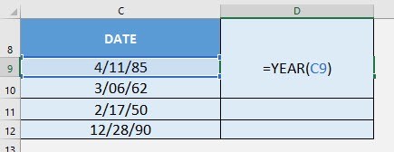 DAY Formula in Excel
Named Ranges
Named ranges can be used to define specific areas of a pivot table and make it easier to reference them in formulas. By using named ranges, you can create formulas that compare values from different pivot tables or different sections of the same table. This is especially useful for calculating custom metrics and identifying specific differences.
3. How To Use The “Show Values As” Option For Comparisons?
To use the “Show Values As” option, right-click on a value field in your pivot table, select “Show Values As,” and then choose a comparison type like “% Difference From.” Specify the base field and item to calculate the difference effectively.
Accessing the Show Values As Option
Right-click on any data cell within the values area of your pivot table. This action opens a context menu with several options.
Select “Show Values As” from the context menu. This opens a submenu with various options for displaying values differently.
Choosing a Comparison Type
From the “Show Values As” submenu, choose a comparison type that suits your needs. Common options include:
- % of Grand Total: Shows each value as a percentage of the entire dataset.
- % of Column Total: Shows each value as a percentage of the column total.
- % of Row Total: Shows each value as a percentage of the row total.
- % Difference From: Calculates the percentage difference from a specified base item.
- Difference From: Calculates the absolute difference from a specified base item.
Specifying the Base Field and Item
If you select “% Difference From” or “Difference From,” a dialog box appears. This dialog box requires you to specify the base field and base item for the calculation.
- Base Field: Choose the field that contains the categories or time periods you want to compare against (e.g., Year, Month, Region).
- Base Item: Select the specific item within the base field that you want to use as the reference point for the comparison (e.g., Previous Year, Specific Month, Particular Region).
Applying the Comparison
Once you have specified the base field and base item, click “OK.” The pivot table updates to display the calculated differences based on your chosen settings.
Interpreting the Results
The pivot table now shows the percentage or absolute differences between each value and the base item. This makes it easier to identify trends, variances, and outliers in your data.
Examples
- Comparing Sales to the Previous Year:
- Select “% Difference From.”
- Base Field: Year.
- Base Item: (previous).
- Comparing Regional Performance to a Specific Region:
- Select “% Difference From.”
- Base Field: Region.
- Base Item: [Specific Region Name].
- Comparing Monthly Performance to a Target:
- Select “Difference From.”
- Base Field: Target.
- Base Item: [Target Value].
Additional Tips
- You can use conditional formatting in combination with “Show Values As” to highlight significant differences.
- Experiment with different comparison types to find the most insightful view of your data.
- Ensure your base field and base item are correctly selected to avoid misleading results.
4. How Does Conditional Formatting Help Highlight Differences?
Conditional formatting allows you to apply visual cues, such as color scales or data bars, to highlight significant differences in your pivot tables. This makes it easier to quickly identify outliers and trends.
Accessing Conditional Formatting
Select the range of cells in your pivot table that you want to format. This is typically the data area where the values are displayed.
Go to the “Home” tab on the Excel ribbon. In the “Styles” group, click on “Conditional Formatting.”
Choosing a Formatting Rule
In the Conditional Formatting menu, you can choose from several rule types:
- Highlight Cells Rules: Highlights cells based on specific criteria, such as greater than, less than, between, or equal to.
- Top/Bottom Rules: Highlights cells in the top or bottom percentile or number range.
- Data Bars: Adds horizontal bars to each cell, visually representing the value relative to other cells.
- Color Scales: Applies a gradient of colors to the cells, indicating the value range.
- Icon Sets: Adds icons to the cells, representing the value category or range.
Applying a Color Scale
Select “Color Scales” from the Conditional Formatting menu. Choose a color scale that suits your needs, such as green-yellow-red or blue-white-red. The colors will be applied to the selected cells, with the highest values represented by one color and the lowest values by another.
Customizing Rules
To customize the formatting rules, select “New Rule” from the Conditional Formatting menu. This allows you to create a rule based on specific criteria, such as a formula or a value range.
In the “New Formatting Rule” dialog box:
- Select “Format only cells that contain.”
- Specify the cell value and condition (e.g., “greater than,” “less than,” “between”).
- Click “Format” to choose the formatting style (e.g., fill color, font color, border).
Managing Rules
To manage existing conditional formatting rules, select “Manage Rules” from the Conditional Formatting menu. This opens the “Conditional Formatting Rules Manager” dialog box.
In the “Rules Manager” dialog box, you can:
- Edit existing rules.
- Delete rules.
- Change the order of rules.
- Apply rules to different ranges of cells.
Examples
- Highlighting Sales Above a Certain Target:
- Select “Highlight Cells Rules” > “Greater Than.”
- Enter the target value.
- Choose a green fill color to indicate values above the target.
- Identifying the Top 10% of Performers:
- Select “Top/Bottom Rules” > “Top 10%.”
- Choose a green fill color to highlight the top performers.
- Using Data Bars to Visualize Sales Performance:
- Select “Data Bars.”
- Choose a data bar style to visually represent sales performance.
Additional Tips
- Use color scales to quickly identify high and low values in your pivot table.
- Use data bars to visualize the relative size of values in your pivot table.
- Use icon sets to categorize values and quickly identify trends.
- Experiment with different formatting rules to find the most effective way to highlight differences in your data.
5. When Should You Use Calculated Fields For Pivot Table Analysis?
Use calculated fields when you need to create new fields based on existing data within your pivot table. This is useful for calculating custom metrics, ratios, or differences that aren’t directly available in the source data.
Defining Calculated Fields
Navigate to the “Analyze” or “Options” tab in the PivotTable Tools section of the Excel ribbon. Click on “Fields, Items, & Sets” and select “Calculated Field.”
Entering the Formula
In the “Insert Calculated Field” dialog box, enter a name for your new field. In the formula box, create a formula using existing fields from your pivot table. You can use mathematical operators (+, -, *, /) and functions (e.g., IF, SUM) to define the calculation.
Adding the Field
Click “Add” to insert the calculated field into your pivot table. The new field will appear in the PivotTable Fields list, allowing you to drag it to the Rows, Columns, or Values area.
Examples
- Calculating Profit Margin:
- Name: Profit Margin.
- Formula: =Sales – Cost.
- Calculating Percentage Change:
- Name: Percentage Change.
- Formula: =(New Value – Old Value) / Old Value.
- Conditional Calculation:
- Name: Performance Status.
- Formula: =IF(Sales > Target, “Exceeded”, “Met”).
Benefits
- Custom Metrics: Create metrics tailored to your specific analysis needs.
- Dynamic Updates: Automatically update calculations when the pivot table data changes.
- Ease of Use: Simplify complex calculations within the pivot table interface.
Considerations
- Complex Formulas: While powerful, complex formulas can make the pivot table harder to understand and maintain.
- Data Source: Calculated fields rely on the existing data in your pivot table; ensure the data source is accurate and complete.
6. What Are The Steps To Calculate Percentage Differences Between Years?
To calculate percentage differences between years, add the sales data to the values area twice, right-click on the second sales column, select “Show Values As” -> “% Difference From,” and set the base field to “Year” and base item to “(previous).”
Prepare Your Data
Ensure your data includes a date column and a sales column. Format the date column correctly so Excel recognizes it as dates.
Create a Pivot Table
Select your data range and insert a pivot table (Insert > PivotTable). Choose where you want the pivot table to be placed.
Add Fields
Drag the following fields to the respective areas:
- Date field to the Rows area.
- Year field (if separate) to the Columns area; if not, group the date field by years.
- Sales field to the Values area twice.
Configure the Percentage Difference
Right-click on any cell in the second “Sum of Sales” column. Select “Show Values As” > “% Difference From.”
In the “Base field” dropdown, select “Year.” In the “Base item” dropdown, select “(previous).” Click “OK.”
Format the Results
The pivot table now displays the percentage difference from the previous year. You can format the numbers as percentages by selecting the data range, right-clicking, and choosing “Format Cells.” In the Format Cells dialog, select “Percentage” and specify the number of decimal places.
Analyze the Data
Review the results to identify trends and changes in sales performance year over year. Use conditional formatting to highlight significant increases or decreases.
Additional Tips
- Add slicers to filter the data by other relevant categories, such as product or region.
- Use pivot charts to visualize the percentage differences and make the data more accessible.
7. How To Group Dates In A Pivot Table For Yearly Comparisons?
Grouping dates allows you to aggregate data by year, quarter, or month, simplifying the comparison process. Right-click on a date in the pivot table, select “Group,” and choose the desired grouping options.
Right-Click on a Date
In your pivot table, right-click on any cell in the date column. This opens a context menu with several options.
Select “Group”
From the context menu, select “Group.” This opens the Grouping dialog box.
Choose Grouping Options
In the Grouping dialog box, you can choose the desired grouping options. For yearly comparisons, select “Years.” You can also select other options like “Months” or “Quarters” to create more granular comparisons.
Specify Starting and Ending Dates
If necessary, specify the starting and ending dates for your grouping. This can be useful if you only want to include data from a specific time period.
Apply the Grouping
Click “OK” to apply the grouping. The pivot table will update to show the data aggregated by the selected grouping options.
Examples
- Grouping by Years: Select “Years” to group the data by calendar years.
- Grouping by Months and Years: Select both “Months” and “Years” to create a hierarchical grouping.
- Grouping by Quarters and Years: Select both “Quarters” and “Years” to compare quarterly performance over multiple years.
Additional Tips
- You can adjust the grouping options at any time by right-clicking on the date column and selecting “Group.”
- Use slicers to filter the data by specific years or time periods.
- Create pivot charts to visualize the grouped data and make comparisons easier.
8. Can You Compare Data From Multiple Excel Sheets In One Pivot Table?
Yes, you can compare data from multiple Excel sheets using Power Query to combine the data into a single source, then create a pivot table from that combined data.
Using Power Query to Combine Data
Open a new Excel workbook or an existing one where you want to create the pivot table. Go to the “Data” tab on the Excel ribbon.
In the “Get & Transform Data” group, click on “From Table/Range” for the first sheet you want to import. This opens the Power Query Editor.
In the Power Query Editor, make any necessary transformations to the data, such as renaming columns or changing data types. Click “Close & Load To” > “Only Create Connection.”
Repeat steps 2-4 for each additional sheet you want to combine.
Appending the Queries
In the “Data” tab, click on “Get Data” > “Combine Queries” > “Append.”
In the Append dialog box, select “Three or more tables.” Add each of the queries you created to the list of tables to append. Click “OK.”
Load the Combined Data
The Power Query Editor opens with the combined data. Review the data to ensure it is correct. Click “Close & Load To” > “Table” to load the combined data into a new sheet.
Create the Pivot Table
Select the combined data range and insert a pivot table (Insert > PivotTable). Choose where you want the pivot table to be placed.
Add Fields and Analyze
Add the relevant fields to the Rows, Columns, and Values areas of the pivot table. Analyze the combined data as needed.
Additional Tips
- Ensure that the columns in each sheet have the same names and data types.
- Use Power Query to clean and transform the data before combining it.
- Add a “Source” column to each sheet to identify the origin of the data.
9. How Can Slicers Enhance Pivot Table Comparisons?
Slicers provide interactive filtering, allowing you to quickly compare specific subsets of data within your pivot tables. This makes it easier to focus on key segments and analyze their differences.
Inserting Slicers
Select any cell within your pivot table. Go to the “Analyze” or “Options” tab in the PivotTable Tools section of the Excel ribbon. Click on “Insert Slicer.”
Choosing Fields
In the “Insert Slicers” dialog box, select the fields you want to use as slicers. These fields should represent categories or attributes that you want to filter the data by (e.g., Region, Product, Year). Click “OK.”
Using Slicers
The slicers appear on the worksheet. Click on the items in the slicers to filter the pivot table data. You can select multiple items by holding down the Ctrl key while clicking.
Examples
- Comparing Sales by Region: Insert a slicer for the “Region” field. Click on different regions to see their respective sales performance.
- Analyzing Product Performance by Year: Insert slicers for both the “Product” and “Year” fields. Filter the data to see how each product performed in different years.
- Viewing Sales by Customer Segment: Insert a slicer for the “Customer Segment” field. Filter the data to compare sales across different customer groups.
Additional Tips
- Use multiple slicers to create complex filters.
- Customize the appearance of slicers by changing their color, font, and layout.
- Connect slicers to multiple pivot tables to filter them simultaneously.
10. What Common Mistakes Should You Avoid When Comparing Pivot Tables?
Common mistakes include comparing data with different granularities, ignoring missing values, and not verifying the accuracy of the source data. Always ensure consistency and validate your data before drawing conclusions.
Comparing Different Granularities
Ensure that the data being compared has the same level of detail. For example, avoid comparing monthly data with quarterly data without proper aggregation.
Ignoring Missing Values
Missing values can skew your comparisons. Handle missing values appropriately by either filling them with a reasonable estimate or excluding them from the analysis.
Not Verifying Source Data Accuracy
Ensure that the source data is accurate and reliable. Errors in the source data will propagate through the pivot tables, leading to incorrect comparisons.
Incorrectly Grouping Data
When grouping dates or other fields, make sure the grouping is done correctly. Incorrect grouping can lead to misinterpretation of the data.
Using Inconsistent Filters
Apply consistent filters across both pivot tables to ensure you are comparing like with like. Inconsistent filters can lead to misleading results.
Misinterpreting Percentage Differences
Understand what the percentage differences are actually representing. A large percentage difference may not be significant if the base value is very small.
Overlooking Contextual Factors
Consider any external factors that may have influenced the data. Changes in market conditions, seasonality, or promotional activities can all affect the results.
Relying Solely on Visualizations
While visualizations can be helpful, don’t rely solely on them. Always verify your findings with numerical data to ensure accuracy.
Failing to Document Your Analysis
Keep a record of your analysis steps, including the data sources, filters, and calculations used. This will help you reproduce the results and ensure consistency over time.
Additional Tips
- Always validate your data before drawing conclusions.
- Use consistent formatting across both pivot tables.
- Consider the limitations of your data and analysis.
COMPARE.EDU.VN provides the resources you need to compare pivot tables effectively, ensuring you gain valuable insights from your data. Address: 333 Comparison Plaza, Choice City, CA 90210, United States. Whatsapp: +1 (626) 555-9090. Visit our website at compare.edu.vn for more information. Let us help you make informed decisions based on thorough data comparison.