Can Excel Compare Two Columns For Differences?

Yes, Excel can adeptly compare two columns for differences. This is a fundamental task in data analysis, and at COMPARE.EDU.VN, we provide expert guidance on leveraging Excel’s features for efficient data comparison, helping you make informed decisions. Master data comparison, identify discrepancies, and ensure data integrity with our comprehensive guide.

1. Understanding the Need to Compare Columns in Excel

Comparing two columns in Excel is a common task with several use cases:

Data Validation: Ensuring data consistency between two datasets.
Duplicate Identification: Finding duplicate entries in a list.
Change Tracking: Identifying changes between two versions of a dataset.
Data Cleaning: Correcting inconsistencies in data.
Decision-Making: Comparing data points to inform decisions.

1.1. Why is Comparing Two Columns Important?

Data accuracy is paramount in any field. Inaccurate data can lead to flawed analysis, poor decision-making, and wasted resources. Comparing two columns allows you to maintain data integrity, ensuring that your information is reliable and consistent. According to a study by the Information Difference, data quality issues cost businesses an estimated $12.9 million annually, highlighting the critical importance of data validation processes.

1.2. Key Benefits of Comparing Columns in Excel

Here are some advantages of comparing columns in Excel:

Improved Data Quality: Identifying and correcting errors.
Time Savings: Automating the comparison process, saving time compared to manual methods.
Better Decision-Making: Ensuring decisions are based on accurate data.
Increased Efficiency: Streamlining data management tasks.
Enhanced Accuracy: Reducing the risk of human error in data entry and analysis.

2. Methods to Compare Two Columns in Excel

Excel offers several methods to compare two columns, each with its own strengths and use cases. Let’s explore these methods:

2.1. Using the IF Function

The IF function is a versatile tool for comparing values in Excel. It allows you to specify a condition and return different values based on whether the condition is true or false.

2.1.1. Syntax of the IF Function

The syntax of the IF function is:

=IF(logical_test, value_if_true, value_if_false)

logical_test: The condition you want to evaluate.
value_if_true: The value to return if the condition is true.
value_if_false: The value to return if the condition is false.

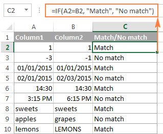
2.1.2. Comparing Columns for Matches

To compare two columns for matches, you can use the IF function to check if the values in corresponding rows are equal. Here’s how:

Enter the Formula: In a new column, enter the following formula in the first row:

=IF(A2=B2, "Match", "No Match")

This formula compares the value in cell A2 with the value in cell B2. If they are equal, it returns “Match”; otherwise, it returns “No Match.”
Drag the Formula: Drag the fill handle (the small square at the bottom-right corner of the cell) down to apply the formula to all rows in the columns.
Review the Results: Examine the new column to see the results of the comparison.

2.1.3. Comparing Columns for Differences

To compare two columns for differences, you can modify the IF function to check if the values in corresponding rows are not equal. Here’s the formula:

=IF(A2<>B2, "Difference", "Same")

This formula returns “Difference” if the values in A2 and B2 are not equal and “Same” if they are equal.

2.2. Using Conditional Formatting

Conditional formatting allows you to highlight cells based on certain criteria. It’s a great way to visually identify matches or differences between two columns.

2.2.1. Highlighting Matches

Here’s how to highlight matches using conditional formatting:

Select the Range: Select the range of cells you want to compare (e.g., A2:A10).
Open Conditional Formatting: Go to the “Home” tab, click on “Conditional Formatting,” and select “New Rule.”
Create a New Rule: Choose “Use a formula to determine which cells to format.”
Enter the Formula: Enter the following formula:

=$A2=$B2

Ensure that the row reference is relative (without the $ sign) like in the formula above.
Set the Format: Click on “Format,” choose a fill color, and click “OK.”
Apply the Rule: Click “OK” to apply the conditional formatting rule.

Now, all cells in column A that match the corresponding cells in column B will be highlighted with the chosen color.

2.2.2. Highlighting Differences

To highlight differences, follow the same steps as above, but use the following formula:

=$A2<>$B2

This will highlight all cells in column A that do not match the corresponding cells in column B.

2.3. Using the EXACT Function

The EXACT function compares two text strings and returns TRUE if they are exactly the same, including case. This is useful for case-sensitive comparisons.

2.3.1. Syntax of the EXACT Function

The syntax of the EXACT function is:

=EXACT(text1, text2)

text1: The first text string to compare.
text2: The second text string to compare.

2.3.2. Comparing Columns for Case-Sensitive Matches

To compare two columns for case-sensitive matches, use the EXACT function in combination with the IF function:

=IF(EXACT(A2, B2), "Match", "No Match")

This formula returns “Match” if the text in cell A2 is exactly the same as the text in cell B2 (including case) and “No Match” otherwise.

2.4. Using COUNTIF for Finding Unique Values

The COUNTIF function counts the number of cells within a range that meet a given criterion. It can be used to find unique values in two columns.

2.4.1. Syntax of the COUNTIF Function

The syntax of the COUNTIF function is:

=COUNTIF(range, criteria)

range: The range of cells to count.
criteria: The condition that must be met for a cell to be counted.

2.4.2. Finding Unique Values in Column A

To find values in column A that are not in column B, use the following formula in a new column:

=IF(COUNTIF($B:$B, A2)=0, "Unique", "")

This formula counts how many times the value in cell A2 appears in column B. If the count is 0, it means the value is unique to column A, and the formula returns “Unique.”

2.4.3. Finding Unique Values in Column B

Similarly, to find values in column B that are not in column A, use the following formula:

=IF(COUNTIF($A:$A, B2)=0, "Unique", "")

This formula counts how many times the value in cell B2 appears in column A. If the count is 0, it means the value is unique to column B, and the formula returns “Unique.”

2.5. Using VLOOKUP or INDEX MATCH

VLOOKUP (Vertical Lookup) and INDEX MATCH are powerful functions for comparing two columns and pulling matching entries from one column to another. VLOOKUP is simpler to use, but INDEX MATCH is more flexible and efficient.

2.5.1. Using VLOOKUP

The VLOOKUP function searches for a value in the first column of a range and returns a value in the same row from another column.

Syntax of the VLOOKUP Function:

=VLOOKUP(lookup_value, table_array, col_index_num, [range_lookup])
lookup_value: The value to search for.
table_array: The range of cells to search in.
col_index_num: The column number in the range from which to return a value.
[range_lookup]: Optional. TRUE for approximate match, FALSE for exact match.
Comparing Columns with VLOOKUP:

To compare the product names in columns D against the names in column A and pull a corresponding sales figure from column B if a match is found, otherwise the #N/A error is returned, use the below formula

=VLOOKUP(D2, $A$2:$B$6, 2, FALSE)

2.5.2. Using INDEX MATCH

The INDEX and MATCH functions are often used together to perform more flexible lookups than VLOOKUP.

Syntax of the INDEX Function:

=INDEX(array, row_num, [column_num])
array: The range of cells to return a value from.
row_num: The row number in the range to return a value from.
[column_num]: Optional. The column number in the range to return a value from.
Syntax of the MATCH Function:

=MATCH(lookup_value, lookup_array, [match_type])
lookup_value: The value to search for.
lookup_array: The range of cells to search in.
[match_type]: Optional. 1 for less than, 0 for exact match, -1 for greater than.
Comparing Columns with INDEX MATCH:

=INDEX($B$2:$B$6, MATCH($D2, $A$2:$A$6, 0))

2.6 Using XLOOKUP

XLOOKUP is a newer function available in Excel 365 and later versions. It combines the capabilities of VLOOKUP and INDEX/MATCH, offering a more versatile and user-friendly way to perform lookups.

2.6.1. Syntax of the XLOOKUP Function

The syntax for XLOOKUP is:

=XLOOKUP(lookup_value, lookup_array, return_array, [if_not_found], [match_mode], [search_mode])

lookup_value: The value to search for.
lookup_array: The range of cells to search in.
return_array: The range of cells to return a value from.
[if_not_found]: Optional. The value to return if no match is found.
[match_mode]: Optional. Specifies the type of match (0 for exact match, -1 for exact match or next smallest, 1 for exact match or next largest, 2 for wildcard match).
[search_mode]: Optional. Specifies the search direction (1 for search from first to last, -1 for search from last to first, 2 for binary search ascending, -2 for binary search descending).

2.6.2. Comparing Columns with XLOOKUP:

=XLOOKUP(D2, $A$2:$A$6, $B$2:$B$6)

3. Advanced Techniques for Column Comparison

Beyond the basic methods, here are some advanced techniques for more complex column comparisons:

3.1. Comparing Multiple Columns

When you need to compare more than two columns, you can extend the IF function or use other functions like AND and OR.

3.1.1. Using AND with IF

To find rows where all columns have the same value, use the AND function within the IF function:

=IF(AND(A2=B2, B2=C2), "Match", "No Match")

This formula returns “Match” only if the values in cells A2, B2, and C2 are all equal.

3.1.2. Using COUNTIF for Multiple Columns

For a more scalable solution, use COUNTIF to check if all columns have the same value:

=IF(COUNTIF($A2:$C2, $A2)=3, "Match", "No Match")

This formula counts how many cells in the range A2:C2 have the same value as A2. If the count is equal to the number of columns being compared (3 in this case), it returns “Match.”

3.2. Case-Insensitive Comparison

If you want to compare text columns without considering case, use the UPPER or LOWER functions to convert the text to the same case before comparing.

3.2.1. Using UPPER

The UPPER function converts a text string to uppercase. Use it like this:

=IF(UPPER(A2)=UPPER(B2), "Match", "No Match")

3.2.2. Using LOWER

The LOWER function converts a text string to lowercase:

=IF(LOWER(A2)=LOWER(B2), "Match", "No Match")

3.3. Comparing Dates

When comparing date columns, ensure that the dates are formatted correctly. Use the DATEVALUE function to convert text dates to numeric dates if necessary.

3.3.1. Using DATEVALUE

The DATEVALUE function converts a text string representing a date to a serial date number:

=IF(DATEVALUE(A2)=DATEVALUE(B2), "Match", "No Match")

4. Practical Examples of Comparing Columns in Excel

Let’s look at some real-world examples of how to compare columns in Excel.

4.1. Example 1: Comparing Customer Lists

Imagine you have two customer lists from different sources, and you want to identify customers who are present in both lists.

Data Preparation: Copy both lists into separate columns in Excel.
Comparison: Use the COUNTIF function to find matching customers:

=IF(COUNTIF($B:$B, A2)>0, "Match", "No Match")

This formula checks if the customer in cell A2 is also present in column B.
Highlighting: Use conditional formatting to highlight the matching customers.

4.2. Example 2: Comparing Product Catalogs

Suppose you have two product catalogs and want to identify products that have different prices in each catalog.

Data Preparation: Copy both catalogs into separate columns in Excel, with product names in one column and prices in another.
Comparison: Use the IF function to compare prices:

=IF(A2<>C2, "Price Difference", "Same Price")

This formula compares the price of the product in cell A2 with the price in cell C2.
Highlighting: Use conditional formatting to highlight the products with price differences.

5. Common Mistakes and How to Avoid Them

When comparing columns in Excel, there are several common mistakes that can lead to inaccurate results. Here’s how to avoid them:

5.1. Incorrect Cell References

Make sure your cell references are correct. Use absolute references ($) when you want to keep a reference fixed and relative references when you want it to change as you copy the formula.

5.2. Ignoring Case Sensitivity

Remember that Excel is case-insensitive by default. Use the EXACT function for case-sensitive comparisons or the UPPER/LOWER functions for case-insensitive comparisons.

5.3. Not Checking Data Types

Ensure that the data types of the columns you are comparing are consistent. Use the VALUE, DATEVALUE, and TEXT functions to convert data types if necessary.

5.4. Overlooking Hidden Characters

Hidden characters, such as spaces or non-printing characters, can cause comparisons to fail. Use the TRIM and CLEAN functions to remove these characters.

5.5. Neglecting Formatting

Formatting differences can also cause comparisons to fail. Use the TEXT function to format numbers and dates consistently before comparing them.

6. Utilizing Excel Add-Ins for Enhanced Comparison

For users seeking a more streamlined and feature-rich experience, Excel add-ins can provide advanced comparison capabilities. One notable tool is the Compare Two Tables add-in, offered as part of the Ultimate Suite by Ablebits.

6.1 Key Features of Compare Two Tables Add-In

Multi-Column Comparison: Compare tables based on multiple columns, enhancing accuracy and relevance.
Duplicate and Unique Value Identification: Easily identify matches (duplicates) and differences (unique values) between lists.
Highlighting and Status Column: Highlight matches or differences with color and insert a status column to label each entry as “Duplicate” or “Unique.”
Customizable Options: Tailor the comparison process to your specific needs with various customizable options.

6.2 Step-by-Step Guide to Using the Add-In

Installation: Install the Ultimate Suite add-in from Ablebits.
Selection: Click the Compare Tables button on the Ablebits Data tab.
Table Definition: Select the first column/list (Table 1) and click Next.
Define Second Table: Select the second column/list (Table 2) and click Next.
Data Type Selection: Choose whether to look for Duplicate values (matches) or Unique values (differences) and click Next.
Column Selection: Select the columns for comparison. For instance, compare “2000 Winners” against “2021 Winners.”
Finalize and Display Results: Choose how to handle the found items (e.g., highlight with color or identify in the Status column) and click Finish.

7. How COMPARE.EDU.VN Simplifies Data Comparison

At COMPARE.EDU.VN, we understand the challenges of data comparison. Our platform is designed to provide you with comprehensive, easy-to-understand guides and tools to make the process as seamless as possible.

7.1. Comprehensive Guides and Tutorials

We offer detailed guides and tutorials on various data comparison techniques in Excel, covering everything from basic functions to advanced methods. Our resources are designed for users of all skill levels, ensuring that everyone can benefit from our expertise.

7.2. Expert Recommendations

Our team of data analysis experts constantly reviews and recommends the best tools and techniques for data comparison. We provide unbiased recommendations based on thorough research and testing, helping you choose the right solutions for your needs.

7.3. User-Friendly Interface

COMPARE.EDU.VN features a user-friendly interface that makes it easy to find the information you need. Our website is organized logically, with clear navigation and a powerful search function, ensuring that you can quickly locate the resources you are looking for.

8. Conclusion: Making Informed Decisions with Data Comparison

Comparing two columns in Excel is a fundamental skill for anyone working with data. By mastering the techniques and avoiding common mistakes, you can ensure that your data is accurate and reliable, leading to better decision-making and increased efficiency.

8.1. Key Takeaways

Use the IF function for simple comparisons.
Apply conditional formatting to highlight matches and differences visually.
Use the EXACT function for case-sensitive comparisons.
Employ COUNTIF for finding unique values.
Leverage VLOOKUP, INDEX MATCH, or XLOOKUP for pulling matching entries.
Avoid common mistakes by checking cell references, data types, and formatting.

8.2. Final Thoughts

Data comparison is not just about identifying differences; it’s about understanding your data and making informed decisions. With the right tools and techniques, you can transform raw data into valuable insights, driving success in your personal and professional endeavors. Visit COMPARE.EDU.VN today to explore our comprehensive resources and take your data comparison skills to the next level.

For more information, feel free to contact us at:

Address: 333 Comparison Plaza, Choice City, CA 90210, United States.

WhatsApp: +1 (626) 555-9090.

Website: COMPARE.EDU.VN

9. Frequently Asked Questions (FAQ)

Q1: How can I compare two columns in Excel for exact matches?

A1: Use the EXACT function in combination with the IF function: =IF(EXACT(A2, B2), "Match", "No Match"). This formula performs a case-sensitive comparison.

Q2: What is the best way to highlight differences between two columns?

A2: Use conditional formatting with the formula =$A2<>$B2. Select the range of cells in column A, go to “Conditional Formatting,” create a new rule using the formula, and choose a fill color to highlight the differences.

Q3: How do I find values in column A that are not present in column B?

A3: Use the COUNTIF function: =IF(COUNTIF($B:$B, A2)=0, "Unique", ""). This formula checks if the value in cell A2 is unique to column A.

Q4: Can I compare two columns without considering case?

A4: Yes, use the UPPER or LOWER functions to convert the text to the same case before comparing: =IF(UPPER(A2)=UPPER(B2), "Match", "No Match").

Q5: How can I compare dates in two columns?

A5: Ensure that the dates are formatted correctly and use the DATEVALUE function if necessary: =IF(DATEVALUE(A2)=DATEVALUE(B2), "Match", "No Match").

Q6: What is the difference between VLOOKUP and INDEX MATCH?

A6: VLOOKUP searches for a value in the first column of a range and returns a value in the same row from another column. INDEX MATCH is more flexible and efficient, allowing you to look up values in any column and return values from any other column.

Q7: How do I compare more than two columns for matches?

A7: Use the AND function with the IF function: =IF(AND(A2=B2, B2=C2), "Match", "No Match"). Alternatively, use COUNTIF: =IF(COUNTIF($A2:$C2, $A2)=3, "Match", "No Match").

Q8: What should I do if my comparisons are failing due to hidden characters?

A8: Use the TRIM and CLEAN functions to remove hidden characters from the cells before comparing them.

Q9: Can I use conditional formatting to highlight rows where all columns have the same value?

A9: Yes, create a conditional formatting rule based on the formula =COUNTIF($A2:$C2, $A2)=3, where 3 is the number of columns to compare.

Q10: Where can I find more detailed guides and expert recommendations for data comparison?

A10: Visit COMPARE.EDU.VN for comprehensive guides, expert recommendations, and user-friendly tools to simplify data comparison in Excel.

By addressing these challenges and providing clear, actionable solutions, compare.edu.vn empowers users to make informed decisions based on accurate and reliable data comparisons. Explore our platform today and unlock the full potential of your data analysis capabilities.