Variances are a fundamental concept in statistics, representing the spread or dispersion of a set of data points around their mean. But Are Variances Comparable across different datasets or scenarios? Understanding variance comparability is crucial for informed decision-making, especially when dealing with different populations, processes, or experimental conditions. This comprehensive guide, brought to you by compare.edu.vn, explores the factors affecting variance comparability and provides practical strategies for accurate analysis and interpretation, enabling you to make confident comparisons. Explore variance analysis, statistical significance, and data interpretation to unlock deeper insights.
Table of Contents
- What is Variance and Why Does It Matter?
- Understanding the Factors Affecting Variance Comparability
- Statistical Tests for Comparing Variances
- When Can You Directly Compare Variances?
- Standardization Techniques for Variance Comparison
- Considering Sample Size and Degrees of Freedom
- The Role of Data Distribution in Variance Analysis
- Interpreting Variance Differences: Practical Significance vs. Statistical Significance
- Common Pitfalls in Variance Comparison and How to Avoid Them
- Case Studies: Real-World Examples of Variance Comparison
- Advanced Techniques for Variance Comparison
- Tools and Software for Variance Analysis
- Best Practices for Reporting Variance Comparisons
- The Future of Variance Analysis
- Frequently Asked Questions (FAQs) About Variance Comparability
1. What is Variance and Why Does It Matter?
Variance is a statistical measure that quantifies the amount of variation or dispersion in a set of data values. A high variance indicates that the data points are spread out over a wide range, while a low variance indicates that the data points are clustered closely around the mean.
Mathematically, variance is calculated as the average of the squared differences from the mean. The formula for the variance of a population is:
σ² = Σ(xᵢ – μ)² / N
Where:
- σ² is the population variance
- xᵢ is each individual data point
- μ is the population mean
- N is the number of data points in the population
- Σ denotes the sum
For a sample, the formula is:
s² = Σ(xᵢ – x̄)² / (n – 1)
Where:
- s² is the sample variance
- xᵢ is each individual data point
- x̄ is the sample mean
- n is the number of data points in the sample
Why does variance matter?
- Understanding Data Spread: Variance provides a clear picture of how spread out the data is, which is essential for understanding the data’s nature.
- Risk Assessment: In finance, variance helps measure the volatility of investments. Higher variance means higher risk.
- Quality Control: In manufacturing, variance is used to ensure consistency in product quality.
- Statistical Inference: Variance is a key component in many statistical tests, such as t-tests and ANOVA, which are used to draw conclusions about populations based on sample data.
- Decision Making: Whether in business, science, or everyday life, understanding variance helps in making informed decisions by considering the range of possible outcomes.
Alt text: Visual representation of variance and standard deviation showing data points spread around the mean.
2. Understanding the Factors Affecting Variance Comparability
When asking “are variances comparable”, it’s important to consider several key factors. Direct comparison of variances can be misleading if these factors are not properly accounted for. These factors include:
2.1. Scale of Measurement
The scale of measurement refers to the type of data being analyzed. There are four main types of scales:
- Nominal: Data are categorized into mutually exclusive, unranked categories (e.g., colors, types of cars).
- Ordinal: Data are ranked in order, but the intervals between values are not necessarily equal (e.g., satisfaction ratings, rankings).
- Interval: Data have equal intervals between values, but there is no true zero point (e.g., temperature in Celsius or Fahrenheit).
- Ratio: Data have equal intervals and a true zero point, allowing for meaningful ratios to be calculated (e.g., height, weight, income).
Variances can only be meaningfully compared for interval and ratio data. Comparing variances of nominal or ordinal data is generally not appropriate because these scales do not provide a consistent numerical basis for calculating dispersion.
2.2. Units of Measurement
The units in which data are measured can significantly affect the magnitude of the variance. For example, measuring height in centimeters will result in a much larger variance than measuring height in meters. To compare variances across different units, it is essential to standardize the data.
2.3. Population Characteristics
Differences in population characteristics can lead to variations in variance. For instance, the variance in income is likely to be higher in a population with a wide range of socioeconomic backgrounds compared to a population with more homogenous income levels.
2.4. Sample Size
The sample size used to estimate the variance can affect the accuracy of the estimate. Smaller sample sizes tend to produce less reliable estimates of variance. It’s crucial to account for sample size when comparing variances, especially when samples are small.
2.5. Data Distribution
The distribution of the data can also impact the interpretation of variance. For example, data that follow a normal distribution will have different variance characteristics compared to data that are skewed or have outliers.
2.6. Presence of Outliers
Outliers, or extreme values, can disproportionately inflate the variance. When comparing variances, it is important to identify and address outliers appropriately, either by removing them (if justified) or by using robust statistical methods that are less sensitive to outliers.
Alt text: Illustrative data distribution showcasing the impact of data spread and outliers on variance calculation.
3. Statistical Tests for Comparing Variances
When you need to determine “are variances comparable”, statistical tests are essential tools to provide an objective and data-driven answer. These tests help you assess whether the differences in variances between two or more groups are statistically significant, considering the inherent variability within the data.
3.1. F-Test
The F-test is a common parametric test used to compare the variances of two populations. It is based on the F-distribution and is sensitive to departures from normality. The F-statistic is calculated as the ratio of the two variances:
F = s₁² / s₂²
Where:
- s₁² is the variance of the first sample
- s₂² is the variance of the second sample
The null hypothesis is that the variances are equal (H₀: σ₁² = σ₂²), and the alternative hypothesis is that they are not equal (H₁: σ₁² ≠ σ₂²). If the calculated F-statistic is significantly different from 1, the null hypothesis is rejected, indicating that the variances are significantly different.
3.2. Levene’s Test
Levene’s test is a more robust alternative to the F-test that does not assume normality. It tests the null hypothesis that the variances of two or more groups are equal. Levene’s test involves transforming the data and performing an ANOVA on the transformed data. The test statistic is less sensitive to departures from normality compared to the F-test.
3.3. Bartlett’s Test
Bartlett’s test is another test for equality of variances, but it is highly sensitive to departures from normality. It is generally recommended to use Levene’s test instead of Bartlett’s test when normality cannot be assumed.
3.4. Chi-Square Test
The Chi-Square test can also be used to compare variances, especially when dealing with categorical data. It examines the differences between observed and expected frequencies to determine if there is a significant difference in the distribution of variances.
3.5. Brown-Forsythe Test
The Brown-Forsythe test is a variant of Levene’s test that uses the median instead of the mean in its calculations, making it even more robust to outliers.
Choosing the Right Test:
- If the data are normally distributed, the F-test is appropriate.
- If the data are not normally distributed, Levene’s test or the Brown-Forsythe test is more suitable.
- For comparing variances across multiple groups, Levene’s test is generally preferred.
Alt text: Diagram illustrating the F-test statistic, used to determine if variances are comparable between two groups.
4. When Can You Directly Compare Variances?
Directly comparing variances is possible under specific conditions. When considering “are variances comparable”, it’s crucial to assess whether these conditions are met to ensure the validity of your comparisons.
4.1. Same Scale of Measurement
The data being compared must be measured on the same scale (e.g., both interval or both ratio scales). Comparing variances across different scales (e.g., comparing the variance of income with the variance of satisfaction ratings) is not meaningful.
4.2. Same Units of Measurement
The data must be measured in the same units. If one dataset is in centimeters and another is in meters, the variances cannot be directly compared without converting to a common unit.
4.3. Similar Populations
The populations from which the data are drawn should be similar in terms of relevant characteristics. For example, comparing the variance of test scores between two classes of students with similar academic backgrounds is more meaningful than comparing the variance between a class of high-achievers and a class of struggling learners.
4.4. Normality Assumption
If using parametric tests like the F-test, the data should be approximately normally distributed. If the normality assumption is violated, non-parametric alternatives like Levene’s test should be used.
4.5. Homogeneity of Variance
Homogeneity of variance, also known as homoscedasticity, means that the variances across different groups are approximately equal. This assumption is important for many statistical tests, such as ANOVA. If variances are not homogenous, corrections or alternative tests may be necessary.
4.6. Independence
The data points within each sample should be independent of each other. If data points are correlated, the variance estimates may be biased.
Example Scenario:
Suppose you are comparing the variances of the heights of male and female students in a university. If both heights are measured in centimeters, the populations are similar, and the data are approximately normally distributed, you can directly compare the variances using an F-test.
Alt text: Illustrative example of homogeneity of variance (equal variance) and heteroscedasticity (unequal variance).
5. Standardization Techniques for Variance Comparison
Standardization is a critical process when directly comparing variances is inappropriate due to differing scales or units of measurement. Standardization techniques transform the data to a common scale, enabling meaningful comparisons.
5.1. Z-Score Standardization
The Z-score, or standard score, measures how many standard deviations each data point is from the mean. The formula for calculating the Z-score is:
Z = (x – μ) / σ
Where:
- x is the individual data point
- μ is the mean of the dataset
- σ is the standard deviation of the dataset
Z-score standardization transforms the data to have a mean of 0 and a standard deviation of 1. This allows for direct comparison of data from different distributions with different scales and units.
5.2. Min-Max Scaling
Min-Max scaling transforms the data to fit within a specific range, typically between 0 and 1. The formula for Min-Max scaling is:
X_scaled = (x – x_min) / (x_max – x_min)
Where:
- x is the individual data point
- x_min is the minimum value in the dataset
- x_max is the maximum value in the dataset
Min-Max scaling is useful when the range of the data is important, and you want to preserve the relationships between the data points.
5.3. Variance Stabilization Transformations
Variance stabilization transformations are used to make the variance of a dataset more constant across different levels of the data. Common transformations include:
- Log Transformation: Useful for data with a right skew and variances that increase with the mean.
- Square Root Transformation: Useful for count data or data with a Poisson distribution.
- Arcsin Transformation: Useful for proportion data.
5.4. Coefficient of Variation (CV)
The coefficient of variation is a relative measure of variability that expresses the standard deviation as a percentage of the mean:
CV = (σ / μ) * 100
The CV is useful for comparing the variability of datasets with different means.
Example Scenario:
Suppose you want to compare the variance of income in two different cities. One city has income measured in USD, and the other has income measured in EUR. To compare the variances, you can convert both datasets to a common currency or use Z-score standardization to remove the effect of the different scales.
Alt text: Formula and explanation of Z-score standardization, a key technique for comparing variances across different scales.
6. Considering Sample Size and Degrees of Freedom
When determining “are variances comparable”, it’s essential to consider the impact of sample size and degrees of freedom on the reliability and interpretation of variance estimates.
6.1. Impact of Sample Size on Variance Estimates
Smaller sample sizes tend to produce less reliable estimates of variance. As the sample size increases, the variance estimate becomes more stable and closer to the true population variance.
6.2. Degrees of Freedom
Degrees of freedom (df) refer to the number of independent pieces of information available to estimate a parameter. In the context of variance, the degrees of freedom are typically n – 1, where n is the sample size.
6.3. Using Degrees of Freedom in Statistical Tests
In statistical tests like the F-test, degrees of freedom are used to determine the critical value and p-value. The degrees of freedom for the F-test are df₁ = n₁ – 1 and df₂ = n₂ – 1, where n₁ and n₂ are the sample sizes of the two groups being compared.
6.4. Adjusting for Sample Size Differences
When comparing variances from samples with different sizes, it is important to consider the impact of sample size on the reliability of the variance estimates. One approach is to use pooled variance, which combines the variance estimates from both samples, weighting them by their degrees of freedom:
s_pooled² = [(n₁ – 1)s₁² + (n₂ – 1)s₂²] / (n₁ + n₂ – 2)
6.5. Confidence Intervals
Confidence intervals provide a range within which the true population variance is likely to fall. Wider confidence intervals indicate greater uncertainty in the variance estimate, often due to smaller sample sizes.
Example Scenario:
Suppose you are comparing the variances of test scores from two schools. School A has a sample size of 30 students, while School B has a sample size of 100 students. The variance estimate from School B will be more reliable due to the larger sample size. When conducting an F-test, you would use df₁ = 29 and df₂ = 99 to determine the p-value.
Alt text: Illustration showing how increasing sample size leads to more accurate and reliable variance estimates.
7. The Role of Data Distribution in Variance Analysis
The distribution of the data plays a crucial role in variance analysis. Whether variances are comparable often depends on the distributional properties of the data being analyzed.
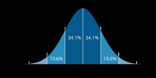
7.1. Normal Distribution
The normal distribution, also known as the Gaussian distribution, is a symmetrical, bell-shaped distribution characterized by its mean and standard deviation. Many statistical tests, such as the F-test, assume that the data are normally distributed.
7.2. Non-Normal Distributions
If the data are not normally distributed, the results of parametric tests like the F-test may be unreliable. In such cases, non-parametric tests like Levene’s test or the Brown-Forsythe test are more appropriate.
7.3. Skewness and Kurtosis
Skewness refers to the asymmetry of the distribution, while kurtosis refers to the peakedness or flatness of the distribution. High skewness or kurtosis can affect the variance and the interpretation of variance comparisons.
7.4. Transformations to Achieve Normality
In some cases, data can be transformed to achieve approximate normality. Common transformations include log transformations, square root transformations, and Box-Cox transformations.
7.5. Outliers
Outliers, or extreme values, can disproportionately inflate the variance. When comparing variances, it is important to identify and address outliers appropriately, either by removing them (if justified) or by using robust statistical methods that are less sensitive to outliers.
Example Scenario:
Suppose you are comparing the variances of income in two different cities. If the income data are highly skewed due to a few very high earners, the F-test may not be appropriate. In this case, you could use a non-parametric test or transform the data to reduce the skewness.
Alt text: Illustration of skewness and kurtosis, demonstrating how these distributional properties affect variance analysis.
8. Interpreting Variance Differences: Practical Significance vs. Statistical Significance
When evaluating “are variances comparable”, it’s essential to differentiate between statistical significance and practical significance. Statistical significance indicates whether the observed difference in variances is likely due to chance, while practical significance assesses whether the difference is meaningful in a real-world context.
8.1. Statistical Significance
Statistical significance is determined by conducting a hypothesis test and calculating a p-value. If the p-value is below a predetermined significance level (e.g., 0.05), the null hypothesis is rejected, and the difference is considered statistically significant.
8.2. Practical Significance
Practical significance refers to the real-world importance or relevance of the observed difference. A statistically significant difference may not be practically significant if the magnitude of the difference is small or if the difference does not have meaningful implications.
8.3. Effect Size
Effect size measures the magnitude of the difference between two groups. Common effect size measures for comparing variances include:
- Cohen’s d: Measures the standardized difference between two means.
- Variance Ratio: The ratio of the two variances being compared.
- Coefficient of Variation (CV): A relative measure of variability that expresses the standard deviation as a percentage of the mean.
8.4. Contextual Considerations
The interpretation of variance differences should always be considered in the context of the specific problem or application. Factors such as the cost of implementing a change, the potential benefits of reducing variance, and the tolerance for variability in the process should be taken into account.
Example Scenario:
Suppose you are comparing the variances of the diameters of two types of bolts. An F-test reveals a statistically significant difference in variances (p < 0.05). However, the variance ratio is only 1.1, meaning that the variance of one type of bolt is only 10% higher than the variance of the other type of bolt. In this case, the difference may not be practically significant if the 10% increase in variance does not have a significant impact on the performance or reliability of the bolts.
Alt text: Visual representation of the difference between statistical significance and practical significance, emphasizing the importance of context.
9. Common Pitfalls in Variance Comparison and How to Avoid Them
When working to understand “are variances comparable”, avoiding common pitfalls is crucial for accurate analysis and decision-making.
9.1. Ignoring the Scale of Measurement
Comparing variances across different scales of measurement (e.g., nominal vs. ratio) is not meaningful and can lead to incorrect conclusions. Always ensure that the data being compared are measured on the same scale.
9.2. Neglecting Units of Measurement
Failing to convert data to a common unit before comparing variances can lead to misleading results. Always convert data to the same units before performing variance comparisons.
9.3. Assuming Normality Without Verification
Many statistical tests assume that the data are normally distributed. Assuming normality without verification can lead to unreliable results. Always check the normality assumption using graphical methods (e.g., histograms, normal probability plots) or statistical tests (e.g., Shapiro-Wilk test, Kolmogorov-Smirnov test).
9.4. Overlooking Outliers
Outliers can disproportionately inflate the variance and distort the results of variance comparisons. Always identify and address outliers appropriately, either by removing them (if justified) or by using robust statistical methods that are less sensitive to outliers.
9.5. Ignoring Sample Size Effects
Smaller sample sizes tend to produce less reliable estimates of variance. Always consider the impact of sample size on the reliability of variance estimates and use appropriate methods for adjusting for sample size differences.
9.6. Confusing Statistical Significance with Practical Significance
A statistically significant difference may not be practically significant if the magnitude of the difference is small or if the difference does not have meaningful implications. Always consider the practical significance of variance differences in the context of the specific problem or application.
9.7. Misinterpreting P-Values
A p-value is the probability of observing a test statistic as extreme as, or more extreme than, the one computed if the null hypothesis is true. A small p-value indicates that the null hypothesis is unlikely to be true, but it does not prove that the alternative hypothesis is true. Avoid overinterpreting p-values and always consider the context of the analysis.
9.8. Data Dredging
Searching for patterns in data without a clear hypothesis can lead to spurious findings. Always formulate a clear hypothesis before conducting variance comparisons and avoid data dredging.
Example Scenario:
Suppose you are comparing the variances of customer satisfaction ratings from two different stores. If you fail to check the normality assumption and the data are highly skewed, you may incorrectly conclude that the variances are significantly different. By checking the normality assumption and using a non-parametric test, you can avoid this pitfall.
Alt text: Infographic highlighting common pitfalls in statistical analysis and how to avoid them, ensuring accurate variance comparison.
10. Case Studies: Real-World Examples of Variance Comparison
To illustrate the practical application of variance comparison, let’s examine a few real-world case studies that demonstrate how assessing “are variances comparable” can inform decision-making and improve outcomes.
10.1. Case Study 1: Manufacturing Quality Control
A manufacturing company produces bolts and needs to ensure that the diameters of the bolts are consistent. The company collects samples of bolts from two different production lines and measures their diameters. The goal is to determine if the variances of the bolt diameters are comparable between the two production lines.
- Data: Diameters of bolts from Production Line A and Production Line B.
- Analysis:
- Check the normality assumption using histograms and normal probability plots.
- Conduct an F-test to compare the variances.
- Calculate the variance ratio to assess the magnitude of the difference.
- Conclusion: If the F-test indicates a statistically significant difference in variances and the variance ratio is high, the company can investigate the production process to identify and address the sources of variability.
10.2. Case Study 2: Investment Portfolio Management
An investor is comparing the volatility of two different stocks to decide which one to include in their portfolio. The investor collects historical price data for both stocks and calculates their variances.
- Data: Historical prices of Stock A and Stock B.
- Analysis:
- Calculate the daily returns for both stocks.
- Calculate the variances of the daily returns.
- Compare the variances to assess the relative volatility of the two stocks.
- Conclusion: If Stock A has a higher variance than Stock B, it is considered more volatile and riskier. The investor can use this information to make informed decisions about their investment strategy.
10.3. Case Study 3: Education Assessment
A school district is comparing the performance of students in two different schools on a standardized test. The district collects test scores from both schools and calculates their variances.
- Data: Test scores from School A and School B.
- Analysis:
- Check the normality assumption using histograms and normal probability plots.
- Conduct an F-test to compare the variances.
- Calculate Cohen’s d to assess the effect size.
- Conclusion: If the F-test indicates a statistically significant difference in variances and Cohen’s d is large, the district can investigate the teaching methods and resources used in the two schools to identify best practices and areas for improvement.
Alt text: Example of a case study applying ANOVA for variance comparison in a real-world scenario.
11. Advanced Techniques for Variance Comparison
Beyond basic statistical tests, advanced techniques provide more sophisticated methods for assessing “are variances comparable”, especially in complex datasets or when dealing with specific research questions.
11.1. Generalized Variance
Generalized variance is a measure of the overall variability of a multivariate dataset. It is calculated as the determinant of the covariance matrix. Generalized variance can be used to compare the variability of two or more multivariate datasets.
11.2. Multivariate Analysis of Variance (MANOVA)
MANOVA is an extension of ANOVA to the case where there are multiple dependent variables. MANOVA can be used to compare the variances of two or more groups on multiple dependent variables simultaneously.
11.3. Bayesian Methods
Bayesian methods provide a framework for incorporating prior knowledge into the analysis of variance. Bayesian methods can be used to estimate the posterior distribution of the variances and to compare the variances of two or more groups.
11.4. Time Series Analysis
Time series analysis is used to analyze data that are collected over time. Time series analysis can be used to compare the variances of two or more time series.
11.5. Spatial Statistics
Spatial statistics is used to analyze data that are collected over space. Spatial statistics can be used to compare the variances of two or more spatial datasets.
Example Scenario:
Suppose you are comparing the variances of multiple dependent variables (e.g., test scores in math, science, and English) between two schools. MANOVA can be used to compare the variances of the three test scores simultaneously.
Alt text: Explanation of MANOVA and its assumptions, used for advanced variance comparison across multiple variables.
12. Tools and Software for Variance Analysis
Several tools and software packages can assist in performing variance analysis, making it easier to determine “are variances comparable” and interpret the results.
12.1. Statistical Software Packages
- R: A free and open-source statistical computing environment with a wide range of packages for variance analysis.
- Python: A versatile programming language with libraries like NumPy, SciPy, and Statsmodels for statistical analysis.
- SAS: A comprehensive statistical software package used in various industries.
- SPSS: A user-friendly statistical software package popular in social sciences and business.
- Minitab: A statistical software package known for its ease of use and quality control tools.
12.2. Spreadsheet Software
- Microsoft Excel: A widely used spreadsheet program with built-in functions for calculating variance and conducting basic statistical tests.
- Google Sheets: A free, web-based spreadsheet program with similar functionality to Excel.
12.3. Online Calculators
- Several online calculators are available for calculating variance and conducting statistical tests. These calculators can be useful for quick and simple analyses.
12.4. Data Visualization Tools
- Tableau: A powerful data visualization tool that can be used to create interactive charts and graphs for exploring variance differences.
- Power BI: A business analytics tool from Microsoft that allows users to visualize data and share insights.
Example Scenario:
Suppose you are using R to compare the variances of two groups. You can use the var.test() function to conduct an F-test and the leveneTest() function from the car package to conduct Levene’s test.
Alt text: Logo of SPSS statistical software, a common tool used for conducting variance analysis.
13. Best Practices for Reporting Variance Comparisons
When reporting the results of variance comparisons, it is important to follow best practices to ensure that the findings are clear, accurate, and reproducible. Transparent reporting enables readers to understand “are variances comparable” in the context of your study.
13.1. Clearly State the Research Question
Clearly state the research question or hypothesis being addressed.
13.2. Describe the Data
Provide a detailed description of the data being analyzed, including the sample size, units of measurement, and any data transformations that were performed.
13.3. Specify the Statistical Methods
Specify the statistical methods used to compare the variances, including the test statistic, degrees of freedom, and p-value.
13.4. Report Effect Sizes
Report effect sizes to provide information about the magnitude of the variance differences.
13.5. Provide Confidence Intervals
Provide confidence intervals for the variance estimates to indicate the uncertainty in the estimates.
13.6. Discuss Assumptions
Discuss any assumptions that were made and provide evidence that the assumptions were met. If the assumptions were not met, discuss the potential impact on the results.
13.7. Interpret the Results in Context
Interpret the results in the context of the specific problem or application. Discuss the practical significance of the variance differences and the implications for decision-making.
13.8. Use Visualizations
Use visualizations, such as box plots or histograms, to illustrate the variance differences.
13.9. Provide a Conclusion
Provide a clear and concise conclusion that summarizes the findings and answers the research question.
Example Scenario:
When reporting the results of an F-test comparing the variances of two groups, you would include the following information:
- “We conducted an F-test to compare the variances of Group A (n = 30, M = 50, SD = 10) and Group B (n = 40, M = 55, SD = 12).”
- “The F-statistic was 1.44, with degrees of freedom 29 and 39. The p-value was 0.21.”
- “The variance ratio was 1.44, indicating that the variance of Group B was 44% higher than the variance of Group A.”
- “The 95% confidence interval for the variance ratio was (0.75, 2.76).”
- “The F-test did not reveal a statistically significant difference in variances between the two groups (p = 0.21).”
- “Therefore, we conclude that there is no evidence to suggest that the variances of Group A and Group B are different.”
Alt text: Overview of best practices for reporting statistical results, ensuring transparency and reproducibility in variance comparisons.
14. The Future of Variance Analysis
The field of variance analysis is continually evolving, with new methods and technologies emerging to address complex data challenges. The future of variance analysis will likely involve:
14.1. Big Data Analytics
The increasing availability of big data is driving the development of new methods for analyzing variance in large and complex datasets.
14.2. Machine Learning
Machine learning algorithms can be used to identify patterns and relationships in data that may not be apparent using traditional statistical methods. Machine learning can also be used to develop predictive models that incorporate variance information.
14.3. Artificial Intelligence (AI)
AI technologies can automate variance analysis tasks, such as outlier detection and data transformation. AI can also assist in the interpretation of variance differences and the identification of actionable insights.
14.4. Cloud Computing
Cloud computing provides access to scalable computing resources and advanced statistical software, making it easier to perform complex variance analyses.
14.5. Real-Time Analytics
Real-time analytics enables the continuous monitoring of variance in dynamic systems, allowing for timely detection of anomalies and proactive intervention.
14.6. Integration with Business Intelligence (BI) Tools
Integration of variance analysis with BI tools allows for seamless incorporation of variance information into business decision-making processes.
Example Scenario:
In the future, AI-powered tools could automatically analyze variance in manufacturing processes, identify potential sources of variability, and recommend corrective actions in real-time, improving product quality and reducing costs.
Alt text: Illustrative depiction of the future of data analytics, highlighting the role of AI and machine learning in variance analysis.
15. Frequently Asked Questions (FAQs) About Variance Comparability
15.1. What does it mean when variances are not comparable?
When variances are not comparable, it means that a direct comparison of their numerical values is not meaningful due to differences in scales, units, populations, or other factors.
15.2. How do I know if I can directly compare variances?
You can directly compare variances if the data are measured on the same scale, in the same units, from similar populations, and the assumptions of the statistical test being used (e.g., normality) are met.
15.3. What should I do if the variances are not comparable?
If the variances are not comparable, you should use standardization techniques to transform the data to a common scale or use non-parametric tests that do not assume equal variances.
15.4. What is the difference between variance and standard deviation?
Variance is a measure of the average squared deviation from the mean, while standard deviation is the square root of the variance. Standard deviation is often preferred because it is in the same units as the original data.
15.5. What is Levene’s test used for?
Levene’s test is used to test the null hypothesis that the variances of two or more groups are equal. It is a robust alternative to the F-test that does not assume normality.
15.6. How does sample size affect variance comparison?
Smaller sample sizes tend to produce less reliable estimates of variance. It is important to consider the impact of sample size on the reliability of variance estimates and use appropriate methods for adjusting for sample size differences.
15.7. What is the practical significance of variance differences?
Practical significance refers to the real-world importance or relevance of the observed variance differences. A statistically significant difference may not be practically significant if the magnitude of the difference is small or if the difference does not have meaningful implications.
15.8. Can I compare variances of categorical data?
No, variances can only be meaningfully compared for interval and ratio data. Comparing variances of nominal or ordinal data is generally not appropriate.
**15.9. What