**How Do I Compare 2 Columns In Excel Sheets Effectively?**

Comparing two columns in Excel sheets doesn’t have to be a daunting task. At COMPARE.EDU.VN, we provide streamlined methods to efficiently compare data, identify matches, and highlight differences. This can be achieved through simple formulas, conditional formatting, or more advanced functions like VLOOKUP, ensuring you can quickly analyze your data and make informed decisions about data comparison and data analysis. Find your comparison solutions on our website.

Table of Contents

1. Why Compare Two Columns In Excel?
2. Methods to Compare Two Columns In Excel
3. Comparing Using the Equals Operator
4. Using IF Conditions for Comparison
5. EXACT() Function for Case-Sensitive Comparisons
6. Conditional Formatting for Highlighting Differences
7. Leveraging Lookup Functions for Data Matching
8. FAQ: Common Questions About Column Comparison
9. Conclusion: Efficient Data Analysis with Excel

1. Why Is It Useful to Compare Two Columns in Excel?

Excel spreadsheets serve as essential tools for data storage, manipulation, and informed decision-making. Excel’s ability to efficiently present and analyze information makes it indispensable for various tasks. Data analysts often rely on Excel to gather critical insights that drive marketing and sales strategies.

When working with large datasets, it’s important to ensure that all cells contain the necessary information for accurate analysis. The absence of data in a cell can significantly impact the outcomes of formulas and tools used. Spreadsheets frequently consist of multiple interconnected files, making manual comparisons a time-consuming and error-prone endeavor. It can take hours or even days to manually sift through the data and pinpoint missing information or discrepancies.

Comparing two columns in Excel enables data analysts to quickly identify whether a cell contains data or not. Excel can display results in various formats, such as TRUE/FALSE, Match/Not Match, or any other user-defined message, providing immediate insights into data consistency and completeness.

2. Methods to Compare Two Columns in Excel

When dealing with data spread across different columns, tables, or even spreadsheets, it’s often necessary to compare them to identify what data is missing or present in both. The approach to comparing two columns should be determined by the specific insights you’re seeking. Here are several methods:

• Highlighting Unique or Duplicate Values: Identify distinct or repeated entries within each column using Excel’s built-in functions.
• Conditional Formatting or Formulas: Apply conditional formatting to visually represent unique or duplicate entries.
• Row-by-Row Comparison: Conduct a direct comparison of values in each row to determine matches or mismatches.
• LOOKUP Formulas: Utilize LOOKUP functions to search for specific values and extract corresponding data for comparison.

By employing these methods, you can efficiently analyze your data and gain meaningful insights.

3. Comparing Using the Equals Operator

Comparing two columns in Excel using the equals operator allows for a straightforward row-by-row analysis, displaying “Match” or “Not Match” results based on whether the data in corresponding rows is identical. The formula =A2=B2 is used to perform this comparison, yielding TRUE if the values match and FALSE if they differ.

To implement this method:

1. In cell C2, enter the formula =A2=B2 and press Enter.
2. Drag the formula down to the end of the table.
3. The formula will return TRUE for rows with matching values and FALSE for rows with differing values.

4. Using IF Conditions for Comparison

Leveraging the IF condition in Excel is an efficient way to compare two columns, returning a specific result based on whether the values match. For instance, the formula =IF(A2=B2,”Match”,””) will display “Match” for rows where the values in columns A and B are identical and leave the cell blank for non-matching rows.

To identify and highlight mismatching values, you can modify the formula to display a different result when the IF condition is false. For example, the formula =IF(A2=B2,”Match”,”Not a Match”) will show “Match” for matching rows and “Not a Match” for mismatching rows.

Additionally, you can use the non-equality sign (<>) to compare two columns and identify differences. The formula =IF(A2<>B2,”Match”,”Not a Match”) will return “Match” for rows where the values in columns A and B are different and “Not a Match” for rows where they are the same.

5. EXACT() Function for Case-Sensitive Comparisons

When comparing two columns in Excel, the EXACT() function is invaluable for performing case-sensitive comparisons. This function ensures that text strings are identical, including their capitalization, before considering them a match. The EXACT() function returns TRUE if the text strings are exactly the same and FALSE otherwise, making it perfect for situations where case sensitivity matters. The syntax is =EXACT(text1, text2), where both text1 and text2 are required arguments.

Here’s how to use the EXACT() function:

1. Enter Your Data: Suppose you have two columns, Data1 and Data2, with text strings like “Nova Scotia” in columns A and B.

2. Apply the Basic Formula: If you use the formula =IF(A2=B2, “Match”, “Mismatch”), Excel will return “Match” because this comparison is case-insensitive.

3. Use the EXACT() Function: To perform a case-sensitive comparison, use the formula =IF(EXACT(A2, B2), “Match”, “Mismatch”).

6. Conditional Formatting for Highlighting Differences

Conditional formatting in Excel is a powerful tool for visually identifying duplicate or unique values in two columns. This method allows you to highlight cells based on whether they meet specific criteria, such as being a duplicate or unique entry. Here’s how to use conditional formatting:

1. Select the Data: Select the entire table or the specific columns you want to compare.

2. Access Conditional Formatting: Go to Home in the Excel ribbon, then click on Conditional Formatting in the Styles group.

3. Choose Highlight Cells Rule: Select Highlight Cells Rules and then choose Duplicate Values.

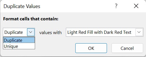
4. Configure the Rule:

   • In the dialog box, you can choose to highlight Duplicate or Unique values from the dropdown menu.
   • Select the formatting style you want to apply (e.g., fill color, text color, or cell border).

7. Leveraging Lookup Functions for Data Matching

Lookup functions in Excel are essential for searching and retrieving data from different parts of a spreadsheet or even different spreadsheets. These functions can help compare two columns by finding matches or identifying missing entries. Excel offers several lookup functions, including HLOOKUP, VLOOKUP, and XLOOKUP. HLOOKUP is used for horizontal lookups, VLOOKUP for vertical lookups, and XLOOKUP, the most versatile, combines features of both.

VLOOKUP Function

The VLOOKUP function is commonly used to compare two columns and find differences. Here’s how to use VLOOKUP to compare columns:

1. Set Up Your Data: Suppose Column A contains a list of exams taken by a student, and Column B lists the subjects the student passed. You want to create a result sheet listing all subjects and indicating whether each was passed.

2. Apply the VLOOKUP Formula: In cell C2, enter the formula =VLOOKUP(A2, $B$2:$B$5, 1, 0). This formula checks if the value in A2 (a subject from the exams list) exists in the range B2:B5 (the list of passed subjects).

3. Drag the Formula: Drag the formula down to apply it to all cells below C2. Column C will show the subjects that were cleared, with #N/A indicating subjects not cleared.

8. FAQ: Common Questions About Column Comparison

1. How to compare two columns in Excel quickly?

To quickly compare two columns in Excel:

1. Select both columns of data.
2. Go to Home → Find & Select → Go To Special → Row Differences.
3. Click OK.

Matching data cells will appear in white, while unmatched cells will be highlighted in gray.

2. What are the other methods to compare two columns in Excel using the IF condition, especially with multiple columns?

When dealing with three or more columns, you can use IF combined with AND or OR to compare data:

• To find matches in all cells within the same row: Use the formula =IF(AND(A2=B2, A2=C2), “Full match”, “”). This formula returns “Full match” if all values in columns A, B, and C of the same row are identical.
• To find matches in any two cells in the same row: Use the formula =IF(OR(A2=B2, B2=C2, A2=C2), “Match”, “”). This formula returns “Match” if any two cells in columns A, B, and C of the same row have the same value.

3. Can you compare two columns in Excel using the Index-Match function?

Yes, the INDEX-MATCH function is an excellent alternative to VLOOKUP for comparing and pulling matching entries from different tables. Here’s how it works:

1. Using MATCH: The MATCH() function compares values in one column (e.g., column D starting from D2) with values in another column (e.g., column A from A2 to A4). It finds the position of the matching value.
2. Using INDEX: If a match is found, the INDEX() function pulls the corresponding value from another column (e.g., column B) and displays it.
3. Handling Non-Matches: If no match is found, the formula returns #N/A.

9. Conclusion: Efficient Data Analysis with Excel

Comparing columns in Excel is a common and crucial task in data analysis. Microsoft Excel provides various methods to compare and match data within single columns, multiple columns, and even across multiple spreadsheets. This guide has shown you several methods to compare two columns for matches and differences.

By mastering these techniques, you can significantly enhance your data analysis skills and make more informed decisions. Remember, for further learning and in-depth tutorials on Excel functions, visit COMPARE.EDU.VN or contact us at:

• Address: 333 Comparison Plaza, Choice City, CA 90210, United States
• WhatsApp: +1 (626) 555-9090
• Website: COMPARE.EDU.VN

Let compare.edu.vn help you unlock the full potential of Excel and data analysis.