How To Compare 3 Columns In Excel Using VLOOKUP?

Comparing data across multiple columns in Excel can be challenging. COMPARE.EDU.VN provides a comprehensive guide on how to effectively use the VLOOKUP function to compare three columns in Excel, offering a streamlined approach to data analysis. This guide will cover the necessary steps and formulas to help you efficiently compare data and identify matches or discrepancies. Explore effective comparison techniques, data matching, and Excel data analysis.

1. Understanding the Basics of VLOOKUP

What is the VLOOKUP Function?

The VLOOKUP function in Excel is a powerful tool used to search for a specific value in the first column of a range, and then return a value from any cell on the same row of that range. According to Microsoft, VLOOKUP is essential for pulling specific data points from large datasets.

Syntax of the VLOOKUP Function

The VLOOKUP function syntax is as follows:

=VLOOKUP(lookup_value, table_array, col_index_num, [range_lookup])

lookup_value: The value you want to search for.
table_array: The range of cells where you want to search.
col_index_num: The column number in the range from which to return a value.
range_lookup: Optional. A logical value (TRUE or FALSE) that specifies whether you want to find an approximate or exact match.

Limitations of Basic VLOOKUP

The basic VLOOKUP function is designed to return a single matching value from one column. This limitation becomes apparent when you need to compare data across multiple columns and extract corresponding values from each.

2. Extending VLOOKUP for Multiple Columns

Using Array Formulas with VLOOKUP

To overcome the single-column limitation, you can use array formulas with VLOOKUP. This allows you to return multiple values from different columns based on a single lookup value.

Syntax for Multiple Column VLOOKUP

The syntax for using VLOOKUP with an array formula to return values from multiple columns is:

=VLOOKUP("lookup_value", lookup_range, {col1, col2, col3...}, [match])

lookup_value: The value you want to look up vertically. Quotes are not used if you reference a cell as a lookup value.
lookup_range: The data range where to search the “lookup_value” and the matching value.
{col1, col2, col3…}: The numbers of the columns that contain the matching values to return. For example, if your range is D7:G18, D is the first column, E is the second one, and so on. You can change the order of columns to the one you need – for example, {5,3,6,2}
match: To return the closest match, specify TRUE; to return the exact match, specify FALSE. The closest match (TRUE) is set by default.

Example: Returning Car, Color, and Country

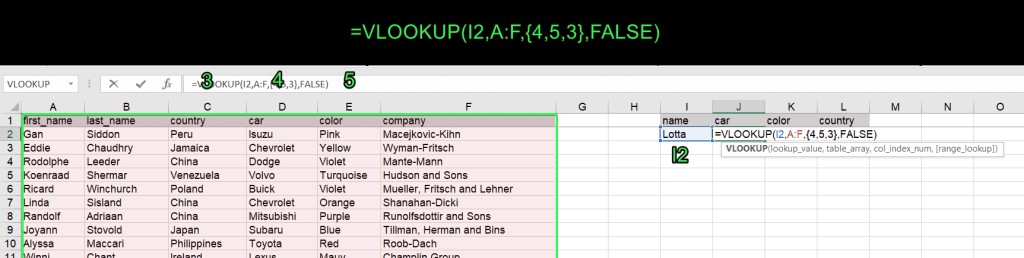
Consider a dataset where you want to find the car, color, and country for a specific user name. The data range is A:F, with the user names in column A, car details in column D, color in column E, and country in column C. The VLOOKUP formula would be:

=VLOOKUP(I2, A:F, {4, 5, 3}, FALSE)

Here, I2 contains the lookup value (user name), A:F is the lookup range, {4, 5, 3} specifies the columns to return (car, color, country), and FALSE ensures an exact match.

Applying the Array Formula

To apply this formula, select a vertical array corresponding to the number of columns in your VLOOKUP formula. In this case, select three cells. After inserting the formula into the formula bar, press Ctrl+Shift+Enter (Windows) or Command+Return (Mac) to apply it as an array formula.

3. Comparing Three Columns Using Nested VLOOKUP

Logic Behind Comparing Three Columns

To compare three columns using VLOOKUP, you need to nest VLOOKUP functions. The logic involves comparing two columns first to identify matches, and then comparing the third column against those matches.

Formula for Comparing Three Columns

The nested VLOOKUP formula for comparing three columns is:

=IFERROR(VLOOKUP(IFERROR(VLOOKUP(A:A, C:C, 1, FALSE),""), E:E, 1, FALSE),"")

VLOOKUP(A:A, C:C, 1, FALSE): Compares columns A (first column) and C (second column).
E:E: The range to look up (third column) against the matching values returned from the comparison of the first and second columns.
1: The column to return the matching values from.
IFERROR: Used to replace #N/A errors with blank cells.

Example: Comparing Old Users, New Users, and Expected Users

Suppose you have three columns: Old Users, New Users, and Expected Users. You want to find the users present in all three columns. The formula will identify values that appear in all three lists.

Implementing the Formula

Select an array that is not less than the arrays in your VLOOKUP formula.
Insert the formula into the formula bar.
Press Ctrl+Shift+Enter (Windows) or Command+Return (Mac) to apply as an array formula.

Excluding Empty Cells

To exclude empty cells, you can use the UNIQUE function (available in Excel 365 or Excel Online) or an advanced array formula:

=IF(ISERROR(SMALL(IF(H2:H66<>"",ROW(H2:H66)-1),ROW(H2:H66)-1)),"", INDEX(H2:H66,MATCH(SMALL(IF(H2:H66<>"",ROW(H2:H66)-1),ROW(H2:H66)-1), IF(H2:H66<>"",ROW(H2:H66)-1),0)))

Replace H2:H66 with your range to apply this formula.

4. VLOOKUP in Excel Online

Simplified Process in Excel Online

Excel Online simplifies the process of using VLOOKUP to return multiple columns. You don’t need to select an array or use Ctrl+Shift+Enter. Just insert the formula in one cell and press Enter. The matching values for the specified columns will populate automatically.

Example in Excel Online

Using the same dataset as before, the VLOOKUP formula in Excel Online would be:

=VLOOKUP(I2, A:F, {4, 5, 3}, FALSE)

Enter this formula in cell J2, and the car, color, and country for the user in cell I2 will be displayed in the adjacent cells.

5. VLOOKUP Across Different Workbooks

Referencing Data in Separate Workbooks

VLOOKUP can also be used to reference data stored in different Excel workbooks. The process is similar, but you need to specify the path to the other workbook in the formula.

Steps to VLOOKUP in a Separate Workbook

Select the array in the target cells where you want the results.
In the formula bar, type =VLOOKUP( and specify the lookup value:
```
=VLOOKUP(A2
```
Enter a comma/semicolon (depending on your regional settings), then click on the spreadsheet with the range you want to look up and select the desired range. The unfinished formula looks like this:
```
=VLOOKUP(A2,[dataset.xlsx]dataset!$A:$F
```
Manually type the range to lookup using the following sample:
```
[dataset.xlsx]dataset!$A:$F
```
- [dataset.xlsx] – name of the spreadsheet
- dataset! – name of the worksheet
- $A:$F – locked range to lookup
Finalize the VLOOKUP formula by entering the numbers of the columns to look up and specifying FALSE for an exact match. Close the bracket and press Ctrl+Shift+Enter (Windows) or Command+Return (Mac).
```
=VLOOKUP(A2,[dataset.xlsx]dataset!$A:$F,{4,5,3},FALSE)
```
Drag the formula down to return matching values for all the users.

6. Common Issues and Troubleshooting

#N/A Error

The #N/A error occurs when VLOOKUP cannot find the lookup value in the specified range.

Solution: Ensure the lookup value exists in the first column of the table array. Check for typos or extra spaces.

Incorrect Column Index Number

If VLOOKUP returns a value from the wrong column, double-check the col_index_num argument.

Solution: Verify that the column number corresponds to the column containing the value you want to retrieve.

Range Lookup Issues

If you are using an approximate match (TRUE), ensure the first column in the table array is sorted in ascending order.

Solution: Sort the first column or switch to an exact match (FALSE) if appropriate.

Array Formula Not Working

If the array formula does not work, make sure you have entered it correctly using Ctrl+Shift+Enter (Windows) or Command+Return (Mac).

Solution: Re-enter the formula, ensuring you press the correct key combination to apply it as an array formula.

7. Alternatives to VLOOKUP

INDEX and MATCH

The INDEX and MATCH functions can be used as a more flexible alternative to VLOOKUP. They can handle lookups in any column and are less sensitive to column insertions or deletions. According to Excel experts, INDEX and MATCH are often preferred for their flexibility.

XLOOKUP

XLOOKUP is a modern replacement for VLOOKUP, offering improved functionality and ease of use. It can handle both vertical and horizontal lookups, and it automatically handles errors.

FILTER Function

The FILTER function allows you to extract data from a range based on specified criteria. This can be useful for comparing columns and returning matching values.

8. Practical Applications

Data Validation

Use VLOOKUP to validate data entries against a master list. For example, ensure that product codes entered in a sales sheet match the product codes in a product catalog.

Merging Data from Different Sources

Combine data from different spreadsheets or databases by using VLOOKUP to match records based on a common identifier.

Financial Analysis

Perform financial analysis by comparing data across different periods or departments, identifying trends and discrepancies.

Inventory Management

Manage inventory by comparing stock levels against sales data, identifying items that need to be reordered.

9. Automating Data Import to Excel

Using Coupler.io

Automating data import to Excel can save significant time and reduce errors. Coupler.io allows you to connect to various data sources and automatically import data into Excel.

Steps to Automate Data Import

Connect your data source and select the data you’d like to export.
Filter and sort it as well as hide, add, and edit columns.
Connect your Microsoft account, specify the Excel workbook, and import your data to it.
Set up a refresh schedule to have your data regularly updated according to the latest changes.

Benefits of Automation

Saves time by eliminating manual data entry.
Reduces errors by automating the data transfer process.
Ensures data is up-to-date with regular refreshes.

10. Conclusion: Mastering VLOOKUP for Data Comparison

Summary of Key Points

Using VLOOKUP to compare three columns in Excel involves understanding the basic VLOOKUP function, extending it with array formulas, and nesting VLOOKUP functions to compare multiple columns. Excel Online simplifies this process, and VLOOKUP can also be used across different workbooks.

Call to Action

Ready to streamline your data analysis process? Visit compare.edu.vn for more in-depth guides and resources on mastering Excel and other data analysis tools. Make informed decisions by leveraging the power of data comparison. Contact us at 333 Comparison Plaza, Choice City, CA 90210, United States, or reach out via WhatsApp at +1 (626) 555-9090.

Final Thoughts

By mastering the techniques outlined in this guide, you can efficiently compare data across multiple columns in Excel, making your data analysis tasks more manageable and effective.

FAQ: Frequently Asked Questions About VLOOKUP

1. Can VLOOKUP compare more than three columns?

Yes, VLOOKUP can compare more than three columns by extending the nested VLOOKUP formula. However, the complexity increases with each additional column.

2. What is the difference between VLOOKUP and HLOOKUP?

VLOOKUP searches vertically in the first column of a range, while HLOOKUP searches horizontally in the first row of a range.

3. How do I fix the #N/A error in VLOOKUP?

Ensure the lookup value exists in the first column of the table array. Check for typos or extra spaces. Use the IFERROR function to handle the error gracefully.

4. Can VLOOKUP return multiple values from different columns?

Yes, by using array formulas, VLOOKUP can return multiple values from different columns.

5. Is XLOOKUP better than VLOOKUP?

XLOOKUP offers improved functionality and ease of use compared to VLOOKUP, including handling both vertical and horizontal lookups and automatic error handling.

6. How do I use VLOOKUP in Google Sheets?

The VLOOKUP function in Google Sheets is similar to Excel. The syntax and functionality are largely the same.

7. What is the purpose of the range_lookup argument in VLOOKUP?

The range_lookup argument specifies whether you want to find an approximate or exact match. TRUE for approximate match, FALSE for exact match.

8. Can I use VLOOKUP to compare data in two different Excel files?

Yes, VLOOKUP can reference data stored in different Excel workbooks. You need to specify the path to the other workbook in the formula.

9. What are some alternatives to VLOOKUP for data comparison?

Alternatives include INDEX and MATCH, XLOOKUP, and the FILTER function.

10. How can I automate data import to Excel?

Use tools like Coupler.io to connect to various data sources and automatically import data into Excel on a scheduled basis.