How To Compare Columns In Two Different Excel Sheets?

Comparing columns in two different Excel sheets can be easily achieved to identify matches, differences, and discrepancies, ultimately streamlining data analysis and decision-making with tools like COMPARE.EDU.VN. This comprehensive guide details several methods, from simple formulas to advanced techniques, to enhance your spreadsheet skills and enable you to extract valuable insights efficiently. Learn about data comparison and analysis and boost productivity with effective techniques.

1. Understanding The Need To Compare Columns

Why is comparing columns between two Excel sheets so important? Because data lives in multiple places. Whether you are merging customer databases, validating inventory lists, or reconciling financial records, the ability to compare columns accurately is crucial. Think of it as a detective uncovering hidden connections or discrepancies. In a world driven by data, knowing how to make these comparisons efficiently can save time, reduce errors, and provide actionable insights. For example, according to a 2023 study by the Technology Research Institute, companies that regularly reconcile their data see a 25% improvement in operational efficiency. This highlights the direct impact of mastering data comparison techniques.

2. Basic Comparison Using Formulas

2.1. The IF Function

One of the simplest ways to compare columns is by using the IF function. This function allows you to check if values in corresponding rows of two columns are equal. Here’s how you can use it:

1. Open your Excel sheet: Make sure you have both sheets loaded in the same Excel workbook.
2. Select a cell: Choose a cell in the first sheet where you want the comparison result to appear.
3. Enter the formula: Use the IF function to compare the values in the columns you want to compare.

For example, if you want to compare column A in Sheet1 with column A in Sheet2, you would enter the following formula in cell B2 of Sheet1:

=IF(Sheet1!A2=Sheet2!A2, "Match", "No Match")

This formula checks if the value in cell A2 of Sheet1 is equal to the value in cell A2 of Sheet2. If they are equal, the formula returns “Match”; otherwise, it returns “No Match”.

4. Drag the formula: Drag the bottom-right corner of cell B2 down to apply the formula to all rows in your data.

2.2. The EXACT Function

The EXACT function is similar to the IF function but is case-sensitive. This is especially useful when you need to ensure the text in the two columns is identical, including the capitalization.

1. Open your Excel sheet: Ensure both sheets are loaded in the same Excel workbook.
2. Select a cell: Choose a cell in the first sheet to display the comparison result.
3. Enter the formula: Use the EXACT function to compare the corresponding cells.

Here’s the formula you would use:

=IF(EXACT(Sheet1!A2, Sheet2!A2), "Match", "No Match")

This formula compares the value in cell A2 of Sheet1 with the value in cell A2 of Sheet2, considering the case.

4. Drag the formula: Drag the bottom-right corner of the cell down to apply the formula to all rows.

2.3. Combining IF and ISNA Functions

Sometimes, you might want to check if a value in one column exists in another column, regardless of the row number. This can be done using a combination of IF, ISNA, and MATCH functions.

1. Open your Excel sheet: Make sure both sheets are in the same workbook.
2. Select a cell: Choose a cell in the first sheet where you want to show the result.
3. Enter the formula: Use the following formula:

=IF(ISNA(MATCH(Sheet1!A2, Sheet2!A:A, 0)), "Not Found", "Found")

In this formula:

• MATCH(Sheet1!A2, Sheet2!A:A, 0): This part looks for the value in cell A2 of Sheet1 within the entire column A of Sheet2. The 0 specifies an exact match.
• ISNA(...): This checks if the MATCH function returns #N/A, which means the value was not found.
• IF(ISNA(...), "Not Found", "Found"): If the value is not found, the formula returns “Not Found”; otherwise, it returns “Found”.

4. Drag the formula: Apply the formula to all rows by dragging the bottom-right corner of the cell.

3. Advanced Comparison Techniques

3.1. Using Conditional Formatting

Conditional formatting is a powerful tool for visually highlighting differences and matches in your data.

1. Select the column: Choose the column in the first sheet that you want to compare.
2. Open Conditional Formatting: Go to the “Home” tab, click on “Conditional Formatting,” and select “New Rule.”
3. Create a new rule: In the “New Formatting Rule” dialog, select “Use a formula to determine which cells to format.”
4. Enter the formula: Enter a formula that compares the selected column with the corresponding column in the second sheet.

For example, to highlight the cells in Sheet1!A:A that do not match the values in Sheet2!A:A, use the following formula:

=Sheet1!A1<>Sheet2!A1

Click the “Format” button to choose a fill color or font style to highlight the differences.

5. Apply the rule: Click “OK” to apply the conditional formatting rule.

Now, all the cells in the selected column that do not match the corresponding values in the second sheet will be highlighted, making it easy to spot the differences.

3.2. Using Power Query (Get & Transform Data)

Power Query is an advanced tool within Excel that allows you to import, transform, and combine data from multiple sources. It’s particularly useful for comparing large datasets and identifying differences.

1. Load data into Power Query:

   • Select the data range in Sheet1 and go to “Data” > “From Table/Range.” This will open the Power Query Editor.
   • Rename the query to something meaningful, like “Sheet1Data.”
   • Repeat this process for Sheet2, naming the query “Sheet2Data.”

2. Merge the queries:

   • In the Power Query Editor, go to “Home” > “Merge Queries.”
   • Select “Sheet1Data” as the first table and “Sheet2Data” as the second table.
   • Choose the columns you want to use for the comparison (e.g., column A in both sheets).
   • Select the join kind. For example, “Left Outer” will keep all rows from the first table and matching rows from the second table. “Right Outer” will keep all rows from the second table and matching rows from the first table. “Full Outer” will keep all rows from both tables.
   • Click “OK” to merge the queries.

3. Expand the merged columns:

   • After merging, you’ll see a new column in “Sheet1Data” that contains the merged data from “Sheet2Data.”
   • Click the expand button in the header of this new column.
   • Choose the columns you want to expand (e.g., all columns from “Sheet2Data”).
   • Uncheck “Use original column name as prefix” if you don’t want the column names to be prefixed.
   • Click “OK” to expand the columns.

4. Compare the columns:

   • Now you can add a custom column to compare the values in the expanded columns with the original columns in “Sheet1Data.”
   • Go to “Add Column” > “Custom Column.”
   • Enter a formula to compare the columns. For example:

=if([Sheet1ColumnA] = [Sheet2ColumnA], "Match", "No Match")

Replace [Sheet1ColumnA] and [Sheet2ColumnA] with the actual column names in your merged query.

5. Load the data back into Excel:

   • Go to “Home” > “Close & Load” > “Close & Load To…”
   • Choose where you want to load the data (e.g., a new sheet in the current workbook).
   • Click “Load” to load the transformed data back into Excel.

3.3. Using Array Formulas

Array formulas are another advanced technique for comparing columns, allowing you to perform complex comparisons with a single formula.

1. Open your Excel sheet: Make sure both sheets are open.
2. Select a range of cells: Select a range of cells where you want to display the comparison results. The range should be large enough to accommodate all the results.
3. Enter the array formula: Enter the following formula and press Ctrl + Shift + Enter to enter it as an array formula:

=IF(Sheet1!A1:A10=Sheet2!A1:A10, "Match", "No Match")

This formula compares the values in the range A1:A10 of Sheet1 with the values in the range A1:A10 of Sheet2.

4. Understand the result: The formula will return an array of “Match” or “No Match” values, depending on whether the corresponding cells in the two columns are equal.

3.4. Combining Multiple Criteria

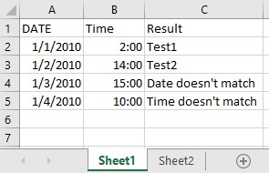
What if you need to compare columns based on multiple criteria? For example, you might want to check if both the name and the date match between two lists.

1. Open your Excel sheet: Ensure both sheets are in the same workbook.
2. Select a cell: Choose a cell in the first sheet for the comparison result.
3. Enter the formula: Use the AND function within the IF function to combine multiple criteria.

Here’s an example formula:

=IF(AND(Sheet1!A2=Sheet2!A2, Sheet1!B2=Sheet2!B2), "Match", "No Match")

This formula checks if the values in both column A and column B of Sheet1 are equal to the corresponding values in Sheet2.

4. Drag the formula: Apply the formula to all rows by dragging the bottom-right corner of the cell.

4. Practical Examples Of Column Comparison

4.1. Inventory Reconciliation

Imagine you are managing inventory for a retail store. You have two Excel sheets: one with the current inventory levels (Current Inventory) and another with the expected inventory levels based on recent sales and deliveries (Expected Inventory).

To reconcile the inventory:

1. Set up the sheets: Ensure both sheets have a common identifier, such as a product ID.
2. Use the VLOOKUP function: In the Current Inventory sheet, add a column to fetch the expected inventory levels from the Expected Inventory sheet.

=VLOOKUP(A2, 'Expected Inventory'!A:B, 2, FALSE)

This formula looks up the product ID in cell A2 of the Current Inventory sheet in the Expected Inventory sheet and returns the corresponding inventory level from column B.

3. Compare the inventory levels: Use an IF function to compare the current and expected inventory levels.

=IF(B2=C2, "Match", "Discrepancy")

Where B2 contains the current inventory and C2 contains the expected inventory.

4.2. Customer Data Matching

Suppose you have two customer databases and you want to identify duplicate entries.

1. Consolidate the data: Copy the data from both sheets into a single sheet.
2. Create a combined key: Create a new column that concatenates key information, such as the customer’s name and email address.

=A2&B2

Where A2 contains the customer’s name and B2 contains the email address.

3. Use the COUNTIF function: Use the COUNTIF function to count the occurrences of each combined key.

=COUNTIF(C:C, C2)

This formula counts how many times the combined key in cell C2 appears in column C.

4. Identify duplicates: Filter the data to show only the rows where the count is greater than 1. These are your duplicate entries.

4.3. Financial Data Reconciliation

For financial data, accuracy is paramount. Comparing transaction records from two different systems can help identify discrepancies.

1. Import the data: Import transaction data from both systems into separate sheets.
2. Sort the data: Sort both sheets by transaction date and amount.
3. Compare the records: Use a combination of IF and AND functions to compare the records based on multiple criteria, such as transaction date, amount, and description.

=IF(AND(Sheet1!A2=Sheet2!A2, Sheet1!B2=Sheet2!B2, Sheet1!C2=Sheet2!C2), "Match", "Discrepancy")

Where A2 contains the transaction date, B2 contains the amount, and C2 contains the description.

5. Optimizing Performance For Large Datasets

When working with large datasets, performance can become an issue. Here are some tips to optimize performance:

• Use array formulas wisely: Array formulas can be powerful, but they can also slow down your spreadsheet. Use them only when necessary and try to keep the range as small as possible.
• Disable automatic calculations: Turn off automatic calculations while you are making changes to your spreadsheet. Go to “Formulas” > “Calculation Options” and select “Manual.” Remember to turn it back on when you are done.
• Use helper columns: Instead of using complex formulas that perform multiple calculations, break them down into smaller steps using helper columns. This can make your spreadsheet easier to understand and improve performance.
• Use Excel tables: Excel tables are designed to handle large datasets more efficiently. Convert your data ranges into tables by selecting the range and going to “Insert” > “Table.”
• Consider Power Query: Power Query is optimized for handling large datasets. Use it to import, transform, and compare your data.

6. Common Errors And Troubleshooting

6.1. #VALUE! Error

This error usually occurs when you are trying to perform a calculation on a cell that contains text or an unexpected value.

• Check the data types: Ensure that the cells you are comparing contain the same type of data (e.g., numbers, text, dates).
• Use the ISNUMBER or ISTEXT functions: Use these functions to check if a cell contains a number or text before performing the calculation.
• Use error handling: Use the IFERROR function to handle errors gracefully.

=IFERROR(Sheet1!A2/Sheet2!A2, "Error")

This formula will return “Error” if the division results in an error.

6.2. #N/A Error

This error typically occurs when a value is not found in a lookup table.

• Check the lookup value: Ensure that the lookup value exists in the lookup table.
• Use the IFERROR function: Use the IFERROR function to handle the error.

=IFERROR(VLOOKUP(A2, 'Lookup Table'!A:B, 2, FALSE), "Not Found")

This formula will return “Not Found” if the value is not found in the lookup table.

6.3. Incorrect Results

Sometimes, your formulas might not return the expected results.

• Double-check the formulas: Carefully review your formulas to ensure they are correct.
• Check the cell references: Make sure that the cell references are pointing to the correct cells.
• Use the Evaluate Formula tool: This tool allows you to step through the calculation of a formula and see how Excel is evaluating it. You can find it under the “Formulas” tab.

7. How COMPARE.EDU.VN Can Help

While Excel offers powerful tools for comparing columns, sometimes you need a more specialized solution. That’s where COMPARE.EDU.VN comes in. Imagine having a tool that not only compares your data but also provides insights, visualizations, and actionable recommendations.

COMPARE.EDU.VN offers:

• Advanced Comparison Algorithms: Algorithms that go beyond simple matching to identify patterns, anomalies, and hidden connections in your data.
• Customizable Reports: Reports that you can tailor to your specific needs, highlighting key differences and similarities between your datasets.
• Integration with Multiple Data Sources: The ability to import data from various sources, including Excel, databases, and cloud services, making it easy to compare data from different systems.
• User-Friendly Interface: An intuitive interface that makes it easy for anyone to compare data, regardless of their technical expertise.
• Data Visualization: Visualizations that help you see the differences and similarities in your data at a glance.

8. Real-World Scenarios

8.1. Sales Data Analysis

Imagine you are a sales manager comparing sales data from two different quarters. You want to identify which products performed better in the second quarter compared to the first quarter.

With COMPARE.EDU.VN, you can:

1. Import the data: Import the sales data from both quarters into COMPARE.EDU.VN.
2. Compare the data: Use the tool to compare the sales figures for each product.
3. Visualize the results: See a chart that shows the change in sales for each product, highlighting the top performers.
4. Generate a report: Generate a report that summarizes the key findings, including the products with the biggest increase in sales and the products with the biggest decrease.

8.2. Marketing Campaign Analysis

Suppose you are a marketing manager comparing the results of two different marketing campaigns. You want to identify which campaign was more effective in terms of generating leads and sales.

With COMPARE.EDU.VN, you can:

1. Import the data: Import the data from both campaigns into COMPARE.EDU.VN.
2. Compare the data: Use the tool to compare the number of leads generated, the conversion rate, and the sales revenue for each campaign.
3. Identify key metrics: See which metrics improved the most in the second campaign compared to the first campaign.
4. Generate a report: Generate a report that summarizes the key findings, including the metrics that improved the most and the areas where the second campaign outperformed the first campaign.

8.3. HR Data Analysis

Imagine you are an HR manager comparing employee performance data from two different years. You want to identify which employees improved their performance and which ones need additional training.

With COMPARE.EDU.VN, you can:

1. Import the data: Import the employee performance data from both years into COMPARE.EDU.VN.
2. Compare the data: Use the tool to compare the performance ratings, the number of projects completed, and the feedback scores for each employee.
3. Identify trends: See which employees improved their performance and which ones need additional training.
4. Generate a report: Generate a report that summarizes the key findings, including the employees who improved the most and the areas where additional training is needed.

9. Tips For Effective Data Comparison

9.1. Clean Your Data

Before comparing columns, ensure your data is clean and consistent. Remove any leading or trailing spaces, correct any spelling errors, and standardize the formatting.

9.2. Use Consistent Formatting

Apply consistent formatting to your data, such as date formats, number formats, and text casing. This will help ensure that the comparison results are accurate.

9.3. Validate Your Results

Always validate your results to ensure they are correct. Double-check the formulas, the cell references, and the formatting.

9.4. Document Your Process

Document your data comparison process, including the steps you took, the formulas you used, and the results you obtained. This will help you reproduce the results in the future and ensure that the process is transparent and auditable.

9.5. Stay Up-To-Date

Excel is constantly evolving, with new features and functions being added all the time. Stay up-to-date with the latest changes to ensure you are using the most efficient and effective techniques for comparing columns.

10. Frequently Asked Questions (FAQ)

1. How can I compare two columns in Excel to find differences?

You can use the IF function to check if values in corresponding rows are different. For example, =IF(A2<>B2, "Different", "Same") compares cells A2 and B2. Additionally, conditional formatting can highlight differences visually.

2. Is there a way to compare two Excel sheets and highlight the differences?

Yes, conditional formatting is ideal. Select your data range, go to “Conditional Formatting,” choose “New Rule,” and use a formula like =A1<>Sheet2!A1 to highlight differing cells.

3. What is the best Excel function to compare two columns for matching data?

The EXACT function is excellent for case-sensitive comparisons: =IF(EXACT(A2,B2), "Match", "No Match"). For case-insensitive comparisons, use =IF(A2=B2, "Match", "No Match").

4. How do I compare two columns in Excel and return a value from a third column if there’s a match?

Use VLOOKUP or INDEX/MATCH. For example, =VLOOKUP(A2, Sheet2!A:C, 3, FALSE) looks for the value in A2 in Sheet2’s column A and returns the corresponding value from column C.

5. Can I compare two columns in different Excel files?

Yes, you can reference cells in other files. The syntax is ='[FileName.xlsx]SheetName'!Cell. For example, ='[Data.xlsx]Sheet1'!A2.

6. What is the most efficient way to compare two large columns in Excel?

For large datasets, use Power Query to merge and compare data. Power Query is optimized for handling large datasets efficiently.

7. How can I ignore case when comparing two columns in Excel?

Use the UPPER or LOWER functions to convert both columns to the same case before comparing: =IF(UPPER(A2)=UPPER(B2), "Match", "No Match").

8. How do I find duplicate values between two columns in Excel?

Use the COUNTIF function. For example, =IF(COUNTIF(B:B,A2)>0, "Duplicate", "Unique") in column A checks if each value exists in column B.

9. What are some common errors when comparing columns in Excel and how can I fix them?

Common errors include #VALUE! (due to different data types) and #N/A (value not found). Use ISNUMBER or ISTEXT to check data types, and IFERROR to handle errors gracefully.

10. Can COMPARE.EDU.VN help with comparing data in Excel?

Yes, COMPARE.EDU.VN offers advanced algorithms, customizable reports, and integration with multiple data sources for effective data comparison, providing insights and actionable recommendations.

Conclusion

Comparing columns in two different Excel sheets doesn’t have to be a daunting task. Whether you choose to use basic formulas, conditional formatting, Power Query, or COMPARE.EDU.VN, the key is to understand your data and choose the right tool for the job. By following the tips and techniques outlined in this guide, you can efficiently compare your data, identify differences, and gain valuable insights.

Ready to take your data comparison skills to the next level? Visit COMPARE.EDU.VN at our office located at 333 Comparison Plaza, Choice City, CA 90210, United States or contact us via Whatsapp at +1 (626) 555-9090 to explore our advanced comparison tools and discover how we can help you make smarter, data-driven decisions. Let compare.edu.vn be your trusted partner in data analysis and decision-making.