How To Compare The Values In Two Columns In Excel?

Comparing values in two columns in Excel is crucial for data analysis, and at COMPARE.EDU.VN, we provide you with simple methods to identify similarities and differences. This guide covers various techniques, from using formulas to conditional formatting, helping you to streamline your data comparison tasks and gain insights quickly. Discover effective ways to compare data sets, find duplicate entries, and ensure data accuracy with our comprehensive guide.

1. Why Is Comparing Two Columns in Excel Important?

Comparing two columns in Excel is important for several reasons, regardless of your profession or industry. Here’s a breakdown of why this skill is invaluable:

Data Validation: Ensuring data accuracy is paramount. Comparing columns helps identify discrepancies, typos, or inconsistencies between datasets. This is vital for maintaining data integrity, especially in finance, healthcare, and research. According to a study by MIT, poor data quality costs organizations an average of $12.9 million annually.
Duplicate Detection: Finding and removing duplicate entries is crucial for cleaning up databases. Duplicate data can skew analysis results and lead to inaccurate conclusions. Comparing columns efficiently pinpoints these redundancies.
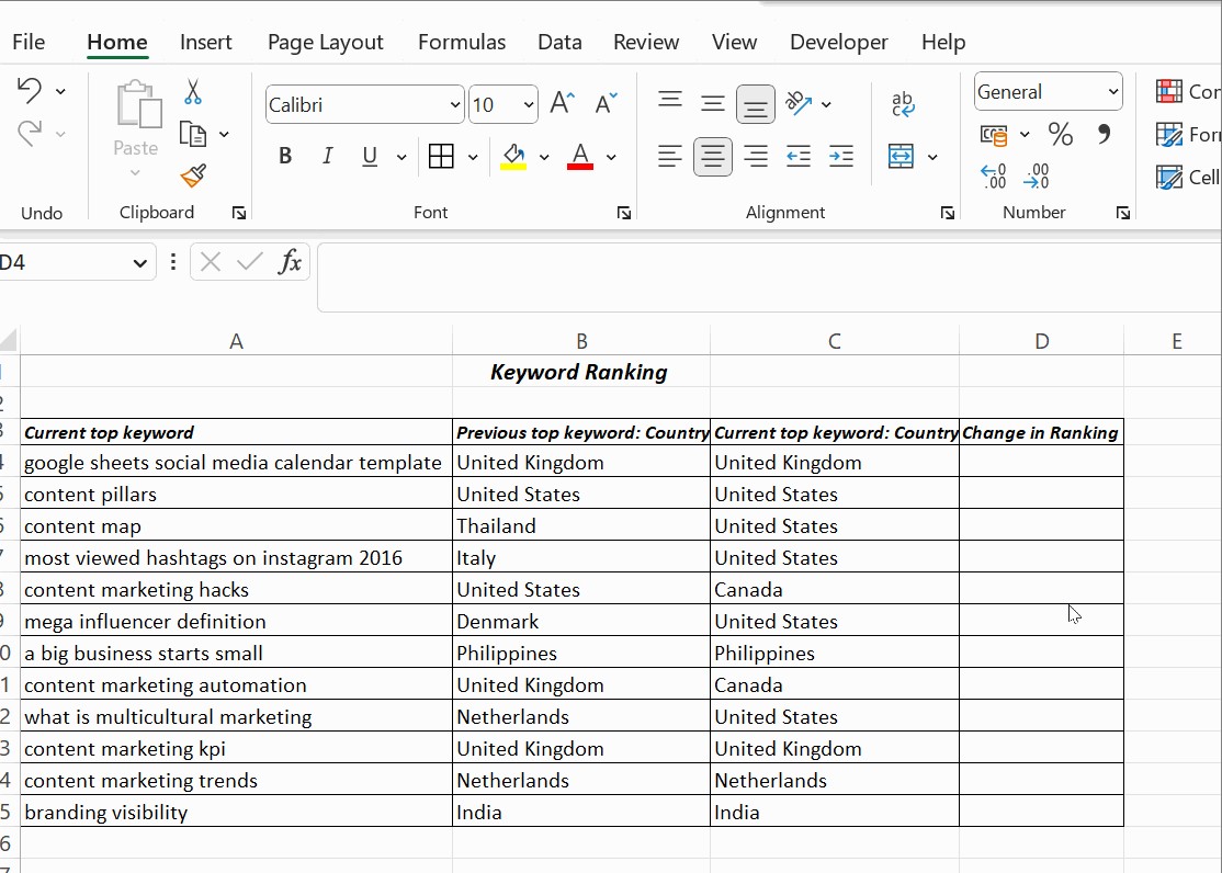
Change Tracking: By comparing historical data with current data, you can track changes and trends over time. This is useful in sales to monitor performance, in inventory management to identify stock fluctuations, and in project management to track task progress.
Data Integration: When merging data from different sources, comparing columns helps ensure consistency and compatibility. This is especially important in large organizations where data silos are common.
Auditing and Compliance: In regulated industries, comparing data against compliance standards or internal policies is essential. This ensures adherence to regulations and helps prevent costly penalties.
Decision Making: Accurate comparisons provide a solid foundation for informed decision-making. Whether it’s choosing between suppliers, evaluating marketing campaigns, or forecasting sales, reliable data comparisons are crucial.

2. What Are the Different Methods to Compare Two Columns in Excel?

Excel offers a variety of methods to compare two columns, each suited to different scenarios and levels of complexity. Here’s a breakdown of the most common techniques:

2.1. Using the Equals Operator (=)

This is the simplest method for a quick, row-by-row comparison. The formula =A1=B1 returns TRUE if the values in cells A1 and B1 are identical, and FALSE otherwise.

Pros: Easy to implement, good for small datasets.
Cons: Doesn’t highlight differences, requires manual review of TRUE/FALSE results.
Best For: Quickly checking if two values in the same row are the same.

2.2. Using the IF Function

The IF function allows you to return custom text based on whether the values match. For example, =IF(A1=B1, "Match", "Mismatch") displays “Match” if the values are the same and “Mismatch” if they are different.

Pros: More informative than the equals operator, easy to understand.
Cons: Still requires manual review, doesn’t highlight differences visually.
Best For: Clearly labeling matching and mismatching rows.

2.3. Using the EXACT Function

The EXACT function is case-sensitive, making it ideal for comparing text strings where capitalization matters. The formula =IF(EXACT(A1, B1), "Match", "Mismatch") will only return “Match” if the values are identical in both content and capitalization.

Pros: Case-sensitive comparison, useful for text-based data.
Cons: Can be too strict in some cases, doesn’t highlight differences visually.
Best For: Situations where capitalization is significant, such as comparing usernames or codes.

2.4. Using Conditional Formatting

Conditional formatting allows you to highlight cells based on specific criteria. You can use it to highlight duplicate or unique values, making it easy to visually identify differences between columns.

Pros: Visual identification of differences, easy to set up.
Cons: Can be overwhelming with large datasets, doesn’t provide specific details about the differences.
Best For: Quickly spotting duplicate or unique entries in two columns.

2.5. Using LOOKUP Functions (VLOOKUP, XLOOKUP)

VLOOKUP and XLOOKUP can be used to find matching values in one column based on values in another. This is useful for comparing lists and identifying missing entries. For example, =VLOOKUP(A1, B:B, 1, FALSE) searches for the value in A1 within column B and returns the corresponding value. If no match is found, it returns an error.

Pros: Powerful for comparing lists and finding missing entries, can return related data.
Cons: Can be complex to set up, requires understanding of lookup functions.
Best For: Comparing large lists and identifying missing or matching items.

3. Step-by-Step Guide: Comparing Two Columns Using the Equals Operator

The equals operator is the most straightforward method for comparing two columns in Excel. Here’s how to use it:

Open your Excel spreadsheet: Ensure that the two columns you want to compare are visible.
Select an empty column: Choose a column next to the columns you are comparing. This column will display the results of the comparison.
Enter the formula: In the first cell of the empty column (e.g., C1), enter the formula =A1=B1. This formula compares the value in cell A1 with the value in cell B1.
Press Enter: Excel will display TRUE if the values in A1 and B1 are the same, and FALSE if they are different.
Apply the formula to the entire column: Click on the bottom-right corner of cell C1 (the small square) and drag it down to the last row of your data. This will apply the formula to all rows, comparing the corresponding cells in columns A and B.
Review the results: Manually scroll through the column to identify rows where the values match (TRUE) or mismatch (FALSE).

4. How to Compare Two Columns Using the IF Function for More Informative Results

While the equals operator provides a basic comparison, the IF function allows you to display more descriptive results. Here’s how to use it:

Open your Excel spreadsheet: Ensure that the two columns you want to compare are visible.
Select an empty column: Choose a column next to the columns you are comparing. This column will display the results of the comparison.
Enter the formula: In the first cell of the empty column (e.g., C1), enter the formula =IF(A1=B1, "Match", "Mismatch"). This formula checks if the value in cell A1 is equal to the value in cell B1. If it is, it displays “Match”; otherwise, it displays “Mismatch”.
Press Enter: Excel will display either “Match” or “Mismatch” based on the comparison.
Apply the formula to the entire column: Click on the bottom-right corner of cell C1 (the small square) and drag it down to the last row of your data. This will apply the formula to all rows, comparing the corresponding cells in columns A and B.
Review the results: Scroll through the column to see which rows have matching values and which have mismatches.

5. Case-Sensitive Comparisons: Using the EXACT Function

In some cases, you may need to perform a case-sensitive comparison. The EXACT function is designed for this purpose. Here’s how to use it:

Open your Excel spreadsheet: Ensure that the two columns you want to compare are visible.
Select an empty column: Choose a column next to the columns you are comparing. This column will display the results of the comparison.
Enter the formula: In the first cell of the empty column (e.g., C1), enter the formula =IF(EXACT(A1, B1), "Match", "Mismatch"). This formula uses the EXACT function to compare the value in cell A1 with the value in cell B1. The EXACT function returns TRUE only if the values are identical, including capitalization.
Press Enter: Excel will display either “Match” or “Mismatch” based on the case-sensitive comparison.
Apply the formula to the entire column: Click on the bottom-right corner of cell C1 (the small square) and drag it down to the last row of your data. This will apply the formula to all rows, comparing the corresponding cells in columns A and B.
Review the results: Scroll through the column to see which rows have matching values and which have mismatches, considering capitalization.

6. How To Compare Columns With Conditional Formatting for Visual Cues

Conditional formatting provides a visual way to compare columns. Here’s how to use it to highlight duplicate or unique values:

Select the columns: Highlight the two columns you want to compare.
Go to Conditional Formatting: On the Home tab, click on Conditional Formatting.
Choose Highlight Cells Rules: Select Highlight Cells Rules from the dropdown menu.
Select Duplicate Values or Unique Values:
- To highlight values that appear in both columns, choose Duplicate Values.
- To highlight values that appear only in one column, choose Unique Values.
Choose a formatting style: In the dialog box, select the formatting style you want to use (e.g., fill color, text color).
Click OK: Excel will highlight the cells that meet the specified criteria.

7. Advanced Comparisons Using LOOKUP Functions (VLOOKUP, XLOOKUP)

LOOKUP functions like VLOOKUP and XLOOKUP are powerful tools for comparing lists and finding missing entries. Here’s how to use VLOOKUP for comparison:

Open your Excel spreadsheet: Ensure that the two lists you want to compare are in separate columns.
Select an empty column: Choose a column next to the first list. This column will display the results of the VLOOKUP function.
Enter the formula: In the first cell of the empty column (e.g., C1), enter the formula =VLOOKUP(A1, B:B, 1, FALSE). This formula searches for the value in cell A1 within column B.
Press Enter:
- If the value in A1 is found in column B, Excel will display the matching value from column B.
- If the value in A1 is not found in column B, Excel will display #N/A.
Apply the formula to the entire column: Click on the bottom-right corner of cell C1 (the small square) and drag it down to the last row of your data. This will apply the formula to all rows, searching for each value in column A within column B.
Identify missing entries: Look for cells that display #N/A. These indicate values in column A that are not present in column B.

Note: XLOOKUP is a more modern and flexible alternative to VLOOKUP. It offers improved performance and can handle more complex scenarios. The XLOOKUP function is available in newer versions of Excel.

8. Real-World Examples of Comparing Columns in Excel

Here are some practical scenarios where comparing columns in Excel can be incredibly useful:

Inventory Management: Compare a list of items received with a list of items ordered to identify discrepancies and ensure accurate stock levels.
Customer Data Analysis: Compare customer lists from different sources to identify duplicate entries and create a unified customer database.
Financial Auditing: Compare transaction records with bank statements to identify unauthorized transactions or errors.
Sales Performance Tracking: Compare sales data from different periods to identify trends and track performance improvements.
HR Management: Compare employee data with payroll records to ensure accurate compensation and benefits.

9. Tips for Efficiently Comparing Columns in Excel

To make your column comparisons more efficient, consider these tips:

Sort your data: Sorting the columns you want to compare can make it easier to spot matches and mismatches.
Use filters: Filters can help you isolate specific values or ranges of values, making it easier to focus on relevant data.
Combine methods: Don’t be afraid to combine different methods to achieve the best results. For example, you can use conditional formatting to highlight differences and then use the IF function to label those differences.
Use helper columns: Sometimes, adding a helper column with a formula can simplify the comparison process.
Automate repetitive tasks: If you frequently perform the same column comparisons, consider creating a macro to automate the process.

10. Common Mistakes to Avoid When Comparing Columns in Excel

Ignoring case sensitivity: Remember that the equals operator and VLOOKUP are not case-sensitive. Use the EXACT function when case matters.
Comparing different data types: Ensure that the columns you are comparing contain the same type of data (e.g., numbers, text, dates).
Not accounting for blank cells: Blank cells can affect the results of your comparisons. Use the ISBLANK function to handle blank cells appropriately.
Using absolute vs. relative references: Be mindful of whether you need to use absolute or relative references in your formulas.
Overlooking hidden rows or columns: Hidden rows or columns can skew your results. Make sure to unhide them before performing your comparisons.

11. Optimizing Performance When Comparing Large Datasets

When working with large datasets, performance can become an issue. Here are some tips to optimize performance:

Use efficient formulas: Some formulas are more efficient than others. For example, XLOOKUP is generally faster than VLOOKUP.
Avoid volatile functions: Volatile functions (e.g., NOW, TODAY, RAND) recalculate every time the worksheet changes, which can slow down performance.
Turn off automatic calculations: Temporarily turning off automatic calculations can speed up the process. Remember to turn them back on when you are finished.
Use array formulas: Array formulas can perform calculations on multiple cells at once, which can be more efficient than using individual formulas.
Consider using Power Query: Power Query is a powerful data transformation tool that can handle large datasets efficiently.

12. Comparing Data Across Multiple Sheets or Workbooks

You can also compare data across multiple sheets or workbooks in Excel. Here’s how:

Referencing cells in other sheets: To reference a cell in another sheet, use the syntax SheetName!CellAddress. For example, Sheet2!A1 refers to cell A1 in Sheet2.
Referencing cells in other workbooks: To reference a cell in another workbook, use the syntax [WorkbookName]SheetName!CellAddress. For example, [Book2]Sheet1!B1 refers to cell B1 in Sheet1 of Book2.
Using the INDIRECT function: The INDIRECT function allows you to dynamically refer to cells in other sheets or workbooks based on a text string. This can be useful when you need to compare data from multiple sources.

13. Alternatives to Excel for Data Comparison

While Excel is a powerful tool for data comparison, there are other options available:

Google Sheets: Google Sheets is a free, web-based spreadsheet program that offers similar functionality to Excel.
специализированное программное обеспечение для сравнения данных: специализированное программное обеспечение для сравнения данных, такое как DiffMerge, Beyond Compare и WinMerge, предназначено для сравнения файлов и папок.
Базы данных: Базы данных, такие как SQL Server, MySQL и PostgreSQL, предлагают расширенные возможности сравнения данных и идеально подходят для больших и сложных наборов данных.
Языки программирования: Языки программирования, такие как Python и R, предлагают гибкие инструменты для сравнения данных и позволяют автоматизировать сложные задачи сравнения.

14. Frequently Asked Questions (FAQ)

1. How can I compare two columns in Excel to find the differences?

You can use the IF function with the not equals operator (<>) to find differences. For example, =IF(A1<>B1, "Different", "Same") will display “Different” if the values in A1 and B1 are not the same.

2. How do I highlight matching values in two columns in Excel?

Use conditional formatting with the “Duplicate Values” rule. Select both columns, go to Home > Conditional Formatting > Highlight Cells Rules > Duplicate Values, and choose a formatting style.

3. Can I compare two columns in Excel for partial matches?

Yes, you can use functions like SEARCH or FIND to check for partial matches. For example, =IF(ISNUMBER(SEARCH(A1, B1)), "Partial Match", "No Match") will check if the value in A1 is a substring of the value in B1.

4. How do I compare two columns and return a value from a third column?

Use the VLOOKUP or XLOOKUP function. For example, =VLOOKUP(A1, B:C, 2, FALSE) will search for the value in A1 within column B and return the corresponding value from column C.

5. How can I ignore errors when comparing two columns in Excel?

Use the IFERROR function to handle errors. For example, =IFERROR(VLOOKUP(A1, B:B, 1, FALSE), "Not Found") will display “Not Found” if the VLOOKUP function returns an error.

6. Is there a way to compare two columns in Excel and count the number of matches?

Yes, you can use the COUNTIF function. For example, =COUNTIF(B:B, A1) will count the number of times the value in A1 appears in column B.

7. How do I compare two date columns in Excel?

You can use the same comparison methods as with other data types. Ensure that the date columns are formatted as dates.

8. Can I compare two columns with different lengths in Excel?

Yes, but you may need to use more advanced techniques, such as dynamic ranges or array formulas, to handle the different lengths.

9. How do I compare two columns and identify missing values?

Use the VLOOKUP or XLOOKUP function. If a value is not found, the function will return an error (#N/A), indicating a missing value.

10. How can I automate the process of comparing two columns in Excel?

Consider using macros or VBA (Visual Basic for Applications) to automate repetitive comparison tasks.

15. Conclusion

Comparing two columns in Excel is a fundamental skill for data analysis and decision-making. Whether you’re validating data, detecting duplicates, or tracking changes, Excel provides a variety of methods to suit your needs. By understanding these techniques and following best practices, you can streamline your data comparison tasks and gain valuable insights.

Ready to take your Excel skills to the next level? Visit COMPARE.EDU.VN for more tutorials, tips, and resources to help you master Excel and other essential software tools.

Contact Us:

Address: 333 Comparison Plaza, Choice City, CA 90210, United States
WhatsApp: +1 (626) 555-9090
Website: COMPARE.EDU.VN

Let compare.edu.vn be your guide to making informed decisions and achieving your goals.