Comparing columns in Excel for differences can be streamlined using various techniques. At COMPARE.EDU.VN, we offer detailed comparisons to help you choose the most efficient methods. Discover the right approach for identifying discrepancies between columns and ensuring data accuracy.
1. Understanding the Importance of Comparing Columns in Excel
Comparing columns in Excel is a crucial skill for data analysis, cleaning, and validation. Whether you are managing customer lists, financial data, or inventory records, the ability to quickly identify differences between columns can save you time and reduce errors. This process ensures data integrity and supports informed decision-making. Let’s dive into several effective methods to compare columns in Excel.
2. Using the IF Function for Row-by-Row Comparison
One of the most basic methods to compare two columns in Excel on a row-by-row basis is by using the IF function. This method allows you to check for matches or differences in each row and return a specified value based on the comparison result.
2.1. Comparing for Matches
To find rows where the content of two cells is identical, you can use the following formula:
=IF(A2=B2,"Match","")This formula checks if the value in cell A2 is equal to the value in cell B2. If they are the same, it returns “Match”; otherwise, it returns an empty string.
2.2. Comparing for Differences
To find rows where the content of two cells is different, you can modify the formula slightly:
=IF(A2<>B2,"No Match","")Here, the <> operator means “not equal to.” If the value in cell A2 is not equal to the value in cell B2, the formula returns “No Match.”
2.3. Combining Matches and Differences
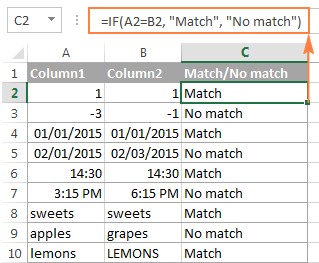
You can also combine the logic to return different values for both matches and differences:
=IF(A2=B2,"Match","No Match")This formula provides a clear indication of whether the cells in each row match or do not match.
3. Case-Sensitive Comparison with the EXACT Function
The IF function, as shown above, ignores case when comparing text values. If you need to perform a case-sensitive comparison, you can use the EXACT function in combination with the IF function.
3.1. Finding Case-Sensitive Matches
To find matches that respect the case of the text, use this formula:
=IF(EXACT(A2,B2),"Match","")The EXACT function returns TRUE if the two text strings are exactly the same, including case, and FALSE otherwise.
3.2. Finding Case-Sensitive Differences
To identify case-sensitive differences, you can modify the formula to return a different value when the strings do not match:
=IF(EXACT(A2,B2),"Match","Unique")In this case, if the strings are not exactly the same, the formula returns “Unique.”
4. Comparing Multiple Columns
When you need to compare more than two columns, you can use combinations of IF, AND, and OR functions. These methods allow you to find matches in all cells or in any two cells within the same row.
4.1. Finding Matches in All Columns
To find rows where all columns have the same values, you can use the AND function:
=IF(AND(A2=B2,A2=C2),"Full Match","")This formula checks if the value in cell A2 is equal to the values in cells B2 and C2. If all conditions are true, it returns “Full Match.”
Alternatively, for tables with many columns, you can use the COUNTIF function:
=IF(COUNTIF($A2:$E2,$A2)=5,"Full Match","")This formula counts how many cells in the range A2 to E2 are equal to the value in cell A2. If the count is 5 (the total number of columns), it returns “Full Match.”
4.2. Finding Matches in Any Two Columns
To find rows where any two columns have the same values, you can use the OR function:
=IF(OR(A2=B2,B2=C2,A2=C2),"Match","")This formula checks if any of the specified conditions are true. If cell A2 equals B2, or B2 equals C2, or A2 equals C2, the formula returns “Match.”
For a more scalable solution with many columns, you can combine multiple COUNTIF functions:
=IF(COUNTIF(B2:D2,A2)+COUNTIF(C2:D2,B2)+(C2=D2)=0,"Unique","Match")This formula checks for any matches between the columns and returns “Match” if any are found; otherwise, it returns “Unique.”
5. Identifying Matches and Differences Between Two Columns
To identify values in column A that are not present in column B, you can use the COUNTIF function.
5.1. Finding Values Unique to Column A
The following formula searches for the value in cell A2 within column B. If no match is found, it returns “No match in B”:
=IF(COUNTIF($B:$B,A2)=0,"No match in B","")This formula checks the entire column B for the value in cell A2. If the count is 0, it means the value is not found in column B.
5.2. Using ISERROR and MATCH Functions
Another way to achieve the same result is by using the ISERROR and MATCH functions:
=IF(ISERROR(MATCH(A2,$B$2:$B$10,0)),"No match in B","")This formula tries to find the value of A2 in the range B2:B10. If the value is not found, the MATCH function returns an error, which ISERROR detects, resulting in “No match in B.”
5.3. Identifying Both Matches and Differences
To identify both matches and differences, you can modify the COUNTIF formula:
=IF(COUNTIF($B:$B,A2)=0,"No match in B","Match in B")This formula now returns “Match in B” if the value in A2 is found in column B.
6. Pulling Matches from Another Table
In scenarios where you need to not only compare columns but also retrieve corresponding data from another table, you can use the VLOOKUP, INDEX MATCH, or XLOOKUP functions.
6.1. Using VLOOKUP
The VLOOKUP function searches for a value in the first column of a range and returns a value from a specified column in the same row.
=VLOOKUP(D2,$A$2:$B$6,2,FALSE)This formula searches for the value in cell D2 within the range A2:B6. If a match is found, it returns the value from the second column (column B) of the same row.
6.2. Using INDEX MATCH
The INDEX MATCH combination is a more flexible alternative to VLOOKUP.
=INDEX($B$2:$B$6,MATCH(D2,$A$2:$A$6,0))This formula first uses MATCH to find the row number where D2 is found in the range A2:A6, and then uses INDEX to return the value from the same row in the range B2:B6.
6.3. Using XLOOKUP
The XLOOKUP function, available in Excel 2021 and Excel 365, is a modern and improved version of VLOOKUP and INDEX MATCH.
=XLOOKUP(D2,$A$2:$A$6,$B$2:$B$6)This formula searches for the value in D2 within the range A2:A6 and returns the corresponding value from the range B2:B6.
For more information, please see How to compare two columns using VLOOKUP.
7. Highlighting Matches and Differences with Conditional Formatting
Conditional formatting allows you to visually highlight cells based on certain criteria. This can be very useful for quickly identifying matches and differences between columns.
7.1. Highlighting Matches and Differences in Each Row
To highlight cells in column A that match the corresponding entries in column B, follow these steps:
- Select the cells in column A.
- Go to Conditional Formatting > New Rule > Use a formula to determine which cells to format.
- Enter the formula
=$B2=$A2. - Choose a format (e.g., fill color) and click OK.
To highlight differences, use the formula =$B2<>$A2.
7.2. Highlighting Unique Entries in Each List
To highlight items that appear in only one list, use the COUNTIF function in a conditional formatting rule.
For unique values in List 1 (column A):
=COUNTIF($C$2:$C$5,A2)=0For unique values in List 2 (column C):
=COUNTIF($A$2:$A$6,C2)=07.3. Highlighting Matches Between Two Columns
To highlight matches between two columns, adjust the COUNTIF formulas to look for counts greater than zero:
For matches in List 1 (column A):
=COUNTIF($C$2:$C$5,A2)>0For matches in List 2 (column C):
=COUNTIF($A$2:$A$6,C2)>08. Highlighting Row Differences and Matches in Multiple Columns
When comparing values in several columns row-by-row, you can quickly highlight matches using conditional formatting and differences using the Go To Special feature.
8.1. Highlighting Rows with Identical Values
To highlight rows that have the same values in all columns, create a conditional formatting rule based on one of the following formulas:
=AND($A2=$B2,$A2=$C2)or
=COUNTIF($A2:$C2,$A2)=38.2. Highlighting Row Differences
To quickly highlight cells with different values in each row, use Excel’s Go To Special feature:
- Select the range of cells you want to compare.
- Go to Home > Editing > Find & Select > Go To Special.
- Select Row differences and click OK.
- The cells whose values are different from the comparison cell in each row will be selected. You can then apply a fill color to highlight them.
9. Comparing Two Cells
Comparing two individual cells is a specific case of comparing two columns row-by-row. You can use the same IF function logic without copying the formula down.
For matches:
=IF(A1=C1,"Match","")For differences:
=IF(A1<>C1,"Difference","")10. Streamlining Column Comparisons with COMPARE.EDU.VN
While Excel provides many built-in functions and features to compare columns, achieving a streamlined and error-free process can still be challenging. At COMPARE.EDU.VN, we understand these challenges and offer comprehensive comparisons of various Excel tools and methods. We aim to provide you with the insights needed to make informed decisions, ensuring efficiency and accuracy in your data analysis tasks.
10.1. Why Choose COMPARE.EDU.VN?
- In-Depth Analysis: We provide detailed comparisons of different Excel techniques and third-party tools, highlighting their strengths and weaknesses.
- Real-World Examples: Our comparisons are based on practical examples and use cases, helping you understand how each method performs in different scenarios.
- User Reviews: We incorporate user reviews and feedback to give you a balanced view of each solution.
- Step-by-Step Guides: We offer step-by-step guides and tutorials to help you implement the recommended methods effectively.
By leveraging the resources at COMPARE.EDU.VN, you can optimize your workflow and ensure the integrity of your data.
11. Frequently Asked Questions (FAQ)
Q1: How do I compare two columns in Excel for exact matches?
A1: Use the formula =IF(EXACT(A2, B2), "Match", "") to compare two columns for case-sensitive matches.
Q2: Can I compare multiple columns for matches in Excel?
A2: Yes, you can use the AND function (e.g., =IF(AND(A2=B2, A2=C2), "Full Match", "")) or the COUNTIF function (e.g., =IF(COUNTIF($A2:$E2, $A2)=5, "Full Match", "") for multiple columns.
Q3: How can I highlight the differences between two columns in Excel?
A3: Use conditional formatting with the formula =$B2<>$A2 to highlight differences between column A and column B.
Q4: What is the best way to find unique values in two different lists in Excel?
A4: Use the COUNTIF function in a conditional formatting rule. For unique values in List 1 (column A), use =COUNTIF($C$2:$C$5, A2)=0.
Q5: How do I compare two columns and pull matching data from another table?
A5: Use the VLOOKUP, INDEX MATCH, or XLOOKUP functions to compare columns and retrieve corresponding data.
Q6: Is there a way to compare two columns in Excel without using formulas?
A6: Yes, you can use Excel add-ins like “Compare Two Tables” from Ablebits Ultimate Suite, which offers a formula-free way to compare and highlight matches or differences.
Q7: How can I compare two columns for differences on a row-by-row basis?
A7: Use the formula =IF(A2<>B2, "No Match", "") to find rows where the content of two cells is different.
Q8: How do I highlight rows that have the same values in several columns?
A8: Create a conditional formatting rule based on the formula =AND($A2=$B2, $A2=$C2) or =COUNTIF($A2:$C2, $A2)=3.
Q9: Can I compare two cells in Excel to see if they match?
A9: Yes, use the formula =IF(A1=C1, "Match", "") to compare two individual cells for matches.
Q10: Where can I find more information on comparing columns in Excel?
A10: Visit COMPARE.EDU.VN for detailed comparisons, real-world examples, and step-by-step guides on various Excel techniques and tools.
12. Conclusion
Comparing columns in Excel is a fundamental skill that can greatly enhance your data management and analysis capabilities. By mastering the techniques outlined in this guide, you can efficiently identify differences, ensure data accuracy, and make informed decisions. For more in-depth comparisons and resources, visit COMPARE.EDU.VN, your trusted source for unbiased and comprehensive evaluations.
Need help making the right choices? Contact us at:
- Address: 333 Comparison Plaza, Choice City, CA 90210, United States
- WhatsApp: +1 (626) 555-9090
- Website: COMPARE.EDU.VN
Visit compare.edu.vn today and discover how easy it can be to make the best decisions for your data needs!