Comparing two rows in Excel and highlighting differences can be streamlined. compare.edu.vn offers detailed guides and tools to simplify this process, ensuring accuracy and efficiency. Explore methods for effective data comparison and difference identification.
1. What Is The Easiest Way To Compare Two Rows In Excel?
The easiest way to compare two rows in Excel is by using a simple formula or conditional formatting. Excel provides several methods to compare data within rows, highlighting matches and differences for clear analysis.
Excel offers several methods to compare data, let’s explore them:
-
Using the IF Function: The IF function is a straightforward way to compare corresponding cells in two rows. You can create a formula that returns “Match” or “No Match” based on whether the cell values are identical.
=IF(A1=A2, "Match", "No Match")This formula compares the values in cells A1 and A2. If they are the same, it returns “Match”; otherwise, it returns “No Match”.
-
Conditional Formatting: Conditional formatting allows you to highlight differences directly in the worksheet. This method is particularly useful for visual comparison.
- Select the two rows you want to compare.
- Go to Home > Conditional Formatting > New Rule.
- Choose “Use a formula to determine which cells to format”.
- Enter the formula
=A1<>A2(assuming A1 is the first cell in your selection). - Click Format to choose a highlight color.
-
The EXACT Function: For case-sensitive comparisons, the EXACT function is invaluable. It ensures that text values match exactly, including capitalization.
=IF(EXACT(A1, A2), "Match", "No Match")This formula compares the values in cells A1 and A2, considering case. It returns “Match” only if the values are identical, including capitalization.
-
Go To Special: The “Go To Special” feature is another quick way to highlight differences.
- Select the rows you want to compare.
- Press F5 or go to Home > Find & Select > Go To Special.
- Select “Row differences” and click OK.
- The cells with differences will be selected. You can then apply a fill color to highlight them.
2. How Can I Compare Two Columns Row-By-Row For Matches?
To compare two columns row-by-row for matches, use the IF function. By applying this formula, you can quickly identify matching entries in corresponding rows.
Here are detailed steps and additional tips to achieve this:
-
Using the IF Function: The IF function is ideal for comparing corresponding cells in two columns and identifying matches.
=IF(A1=B1, "Match", "No Match")This formula compares the values in cells A1 and B1. If they are the same, it returns “Match”; otherwise, it returns “No Match”.
-
Drag the Formula Down: After entering the formula in the first row, drag the fill handle (the small square at the bottom-right corner of the cell) down to apply the formula to the remaining rows. This automatically adjusts the cell references for each row.
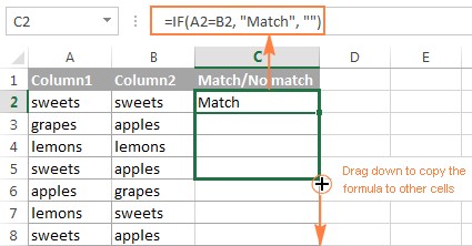 Copy the formula down to other cells to compare two columns in Excel.
-
Conditional Formatting for Visuals: For a visual representation, use conditional formatting to highlight matches.
- Select the range of cells in both columns.
- Go to Home > Conditional Formatting > New Rule.
- Choose “Use a formula to determine which cells to format”.
- Enter the formula
=$A1=$B1(assuming A1 is the first cell in your selection). - Click Format to choose a highlight color for matches.
-
Combining IF and Conditional Formatting: You can combine the IF function and conditional formatting for a more detailed analysis. Use the IF function to create a new column indicating matches, then use conditional formatting to highlight these matches.
-
Using the EXACT Function: For case-sensitive comparisons, use the EXACT function within the IF formula:
=IF(EXACT(A1, B1), "Match", "No Match")This ensures that only exact matches (including capitalization) are identified.
-
Compare Numbers, Dates, and Text: The basic IF formula works well for numbers, dates, and text. Excel automatically recognizes the data type and performs the comparison accordingly.
-
Named Ranges for Clarity: Use named ranges to make your formulas more readable. For example, if column A contains “Names1” and column B contains “Names2”, the formula becomes:
=IF(Names1=Names2, "Match", "No Match")
This makes it easier to understand and maintain.
-
Handling Errors: If your data contains errors (e.g., #N/A), use the IFERROR function to handle them gracefully.
=IFERROR(IF(A1=B1, "Match", "No Match"), "Error")
This prevents errors from disrupting your comparison.
-
Advanced Filtering: Use advanced filtering to display only the rows that match or do not match.
- Go to the Data tab and click on Advanced.
- Set up your criteria range with headers that match your data (e.g., “Column A”, “Column B”) and enter the formula
=A1=B1under the headers. - Choose to filter the list in-place or copy the results to another location.
3. How Do I Highlight Differences Between Two Rows In Excel?
Highlighting differences between two rows in Excel can be achieved using conditional formatting. By setting up a rule, you can automatically highlight cells with different values.
Here’s a comprehensive guide:
-
Using Conditional Formatting: Conditional formatting is the most efficient way to highlight differences between two rows.
- Select the Rows: Select the range of cells in the rows you want to compare. For example, select A1:Z1 and A2:Z2 if you want to compare the first two rows across columns A to Z.
- Open Conditional Formatting: Go to Home > Conditional Formatting > New Rule.
- Choose a Rule Type: Select “Use a formula to determine which cells to format”.
- Enter the Formula: Enter the following formula:
=A1<>A2Ensure that the cell references are relative (without the $ sign) so that the formula adjusts correctly for each cell in the selected range.
5. Set the Format: Click on the Format button, go to the Fill tab, and choose a highlight color. Click OK to close the Format dialog and OK again to create the rule. -
Understanding the Formula: The formula
A1<>A2checks if the value in cell A1 is not equal to the value in cell A2. If the values are different, the formula returns TRUE, and the conditional formatting is applied. -
Applying to Multiple Rows: If you need to compare multiple pairs of rows (e.g., rows 1 and 2, rows 3 and 4, etc.), you can adjust the formula slightly and use the Format Painter to apply the formatting to other row pairs.
- Select the formatted rows.
- Click the Format Painter icon in the Home tab.
- Select the next pair of rows you want to format.
-
Using the EXACT Function for Case-Sensitive Differences: If you need to consider case when comparing text values, use the EXACT function within the conditional formatting formula:
=NOT(EXACT(A1,A2))This formula checks if the values in cells A1 and A2 are not exactly the same (including case).
-
Highlighting Entire Rows Based on Differences: To highlight the entire row if any difference exists, modify the formula to check all relevant columns and apply the formatting to the entire row.
- Select the entire row.
- Create a new conditional formatting rule using the formula:
=OR(A1<>A2, B1<>B2, C1<>C2, ...)Replace A1, B1, C1, etc., with the first cell in each column you want to compare.
-
Using Helper Columns: You can also use a helper column to identify differences and then use conditional formatting based on the helper column.
- In a helper column (e.g., column C), enter the formula:
=IF(A1<>A2, "Difference", "")- Drag the formula down to apply it to all rows.
- Select the data range (including the helper column).
- Create a conditional formatting rule that highlights cells where the helper column contains “Difference”.
-
Highlighting Based on Multiple Conditions: You can combine multiple conditions in your conditional formatting formula. For example, you might want to highlight cells that are different and also meet another criterion.
=AND(A1<>A2, A1>10)This formula highlights cells that are different and have a value greater than 10.
-
Color Scales for Visual Analysis: Use color scales to create a visual gradient based on the degree of difference between values.
- Select the range of cells.
- Go to Home > Conditional Formatting > Color Scales.
- Choose a color scale that suits your needs.
-
Managing Conditional Formatting Rules: To manage, edit, or delete conditional formatting rules, go to Home > Conditional Formatting > Manage Rules.
4. Can I Use Formulas To Identify Differences?
Yes, formulas can effectively identify differences between two rows in Excel. Using functions like IF and EXACT, you can pinpoint specific discrepancies in your data.
Here’s how you can use formulas to identify differences:
-
Using the IF Function: The IF function is a simple yet powerful way to identify differences. You can set up a formula to return a specific value (e.g., “Difference”) when two cells are not equal.
=IF(A1<>B1, "Difference", "")This formula compares the values in cells A1 and B1. If they are different, it returns “Difference”; otherwise, it returns an empty string.
-
Using the EXACT Function for Case-Sensitive Comparisons: For text values, the EXACT function ensures that the comparison is case-sensitive.
=IF(EXACT(A1, B1), "", "Case Difference")This formula checks if the values in cells A1 and B1 are exactly the same (including case). If they are not, it returns “Case Difference”.
-
Combining IF and ISBLANK: To handle blank cells, combine the IF and ISBLANK functions.
=IF(AND(ISBLANK(A1), ISBLANK(B1)), "", IF(A1<>B1, "Difference", ""))This formula checks if both cells A1 and B1 are blank. If they are, it returns an empty string. If not, it compares the values and returns “Difference” if they are different.
-
Using a Helper Column: A helper column can simplify complex comparisons.
- In a helper column (e.g., column C), enter the formula:
=IF(A1<>B1, "Difference", "")- Drag the formula down to apply it to all rows.
- You can then filter or sort the helper column to quickly identify rows with differences.
-
Using the XOR (Exclusive OR) Logic: The XOR logic can be useful when you want to identify rows where only one of the cells has a value. However, Excel doesn’t have a built-in XOR function. You can simulate it using a combination of AND and OR:
=IF(OR(AND(A1<>"", B1=""), AND(A1="", B1<>"")), "XOR", "")This formula checks if either A1 has a value and B1 is blank, or A1 is blank and B1 has a value. If either condition is true, it returns “XOR”.
-
Comparing Multiple Columns: To compare multiple columns, you can nest IF functions or use the AND function:
=IF(AND(A1=B1, B1=C1), "Match", "Difference")This formula checks if the values in cells A1, B1, and C1 are all the same. If they are, it returns “Match”; otherwise, it returns “Difference”.
-
Finding the Specific Difference: To identify the specific difference between two numeric values, you can use a simple subtraction formula:
=A1-B1This formula returns the difference between the values in cells A1 and B1.
-
Handling Different Data Types: Ensure that the data types in the cells you are comparing are consistent. If you are comparing a number to text, Excel may not return the expected results. Use functions like VALUE or TEXT to convert data types if necessary.
=IF(VALUE(A1)=VALUE(B1), "Match", "Difference")
This formula converts the values in cells A1 and B1 to numbers before comparing them.
5. How Do I Quickly Find Discrepancies In Large Datasets?
To quickly find discrepancies in large datasets, leverage Excel’s powerful features such as conditional formatting, filtering, and formulas. These tools can help you efficiently identify and highlight inconsistencies.
Here’s a detailed approach:
-
Conditional Formatting: Use conditional formatting to highlight discrepancies based on specific criteria.
-
Highlight Duplicate Values:
- Select the column or range.
- Go to Home > Conditional Formatting > Highlight Cells Rules > Duplicate Values.
- Choose the formatting style (e.g., fill color) and click OK.
-
Highlight Unique Values:
- Select the column or range.
- Go to Home > Conditional Formatting > Highlight Cells Rules > Duplicate Values.
- Change the selection to “Unique” and choose the formatting style.
-
Highlight Cells Based on a Formula:
- Select the range of cells.
- Go to Home > Conditional Formatting > New Rule.
- Select “Use a formula to determine which cells to format”.
- Enter a formula that identifies the discrepancy (e.g.,
=A1<>B1to highlight differences between columns A and B). - Choose the formatting style and click OK.
-
-
Filtering: Use filtering to narrow down your dataset and focus on specific discrepancies.
-
Enable Filtering:
- Select the header row.
- Go to Data > Filter.
-
Filter by Criteria:
- Click the filter arrow in the column you want to filter.
- Use the available options (e.g., “Number Filters”, “Text Filters”, “Date Filters”) to set your criteria.
- You can also use “Custom Filter” for more complex conditions.
-
Filter by Cell Color:
- If you’ve used conditional formatting, you can filter by cell color to isolate highlighted discrepancies.
- Click the filter arrow, go to “Filter by Color”, and select the color you want to filter.
-
-
Formulas: Use formulas to create helper columns that identify discrepancies.
-
Compare Two Columns:
- In a helper column (e.g., column C), enter the formula:
=IF(A1<>B1, "Difference", "")- Drag the formula down to apply it to all rows.
- Filter the helper column to show only rows with “Difference”.
-
Check for Blank Cells:
- In a helper column, enter the formula:
=IF(ISBLANK(A1), "Blank", "")- Filter the helper column to show only rows with “Blank”.
-
Calculate Differences:
- In a helper column, enter the formula:
=A1-B1- Use conditional formatting to highlight significant differences (e.g., values greater than a certain threshold).
-
-
Pivot Tables: Use pivot tables to summarize and analyze your data, making it easier to spot discrepancies.
-
Create a Pivot Table:
- Select your data range.
- Go to Insert > PivotTable.
- Choose where to place the pivot table and click OK.
-
Analyze Your Data:
- Drag fields into the “Rows”, “Columns”, and “Values” areas to summarize your data.
- Use pivot table features like grouping, sorting, and filtering to identify discrepancies.
-
-
Data Validation: Use data validation to prevent discrepancies from occurring in the first place.
-
Set Up Data Validation:
- Select the cells you want to validate.
- Go to Data > Data Validation.
- Choose the validation criteria (e.g., “Whole number”, “Decimal”, “List”, “Date”, “Text length”).
- Set the appropriate settings (e.g., minimum and maximum values).
-
Create an Error Alert:
- Go to the “Error Alert” tab in the Data Validation dialog.
- Customize the error message that appears when invalid data is entered.
-
-
Excel Add-Ins: Consider using Excel add-ins designed for data cleaning and analysis. These add-ins often provide advanced features for identifying and correcting discrepancies.
-
Go To Special: Use the “Go To Special” feature to quickly select cells with specific characteristics.
-
Select the Range:
- Select the range of cells you want to analyze.
-
Open Go To Special:
- Press F5 or go to Home > Find & Select > Go To Special.
-
Choose a Special Type:
- Select the type of cells you want to select (e.g., “Blanks”, “Constants”, “Formulas”, “Row differences”, “Column differences”).
- Click OK.
-
Highlight or Filter:
- Once the cells are selected, you can highlight them using conditional formatting or filter the data to show only those cells.
-
-
Auditing Tools: Use Excel’s auditing tools to trace the relationships between cells and formulas. This can help you identify the source of discrepancies.
-
Show Formulas:
- Go to the Formulas tab and click “Show Formulas” to display all formulas in the worksheet.
-
Trace Precedents and Dependents:
- Select a cell and click “Trace Precedents” or “Trace Dependents” to see which cells are used in the formula or which cells depend on the selected cell.
-
Error Checking:
- Use the “Error Checking” tool to identify common errors in your formulas.
-
6. How Can VLOOKUP Help In Comparing Rows?
VLOOKUP can help compare rows by searching for values in one row within another. This is particularly useful when identifying if a specific entry exists in a different row.
Here’s how VLOOKUP can be utilized effectively:
-
Basic VLOOKUP Syntax: VLOOKUP searches for a value in the first column of a range and returns a value from a specified column in the same row. The syntax is:
=VLOOKUP(lookup_value, table_array, col_index_num, [range_lookup])- lookup_value: The value you want to find.
- table_array: The range in which to search.
- col_index_num: The column number in the range from which to return a value.
- [range_lookup]: TRUE for approximate match (not recommended for comparisons); FALSE for exact match.
-
Comparing Rows Using VLOOKUP: To compare two rows, you can use VLOOKUP to check if values from one row exist in another.
-
Set Up Your Data: Suppose you have two rows of data you want to compare:
- Row 1: A1, B1, C1, D1
- Row 2: A2, B2, C2, D2
-
Use VLOOKUP to Check for Matches: In a helper column, use VLOOKUP to search for each value from Row 1 in Row 2. For example, in cell A3, enter the formula:
=IF(ISNA(VLOOKUP(A1, $A$2:$D$2, 1, FALSE)), "Not Found", "Found")This formula searches for the value in A1 within the range A2:D2 (Row 2). If the value is found, VLOOKUP returns the value; otherwise, it returns #N/A. The ISNA function checks if VLOOKUP returns #N/A. If it does, the formula returns “Not Found”; otherwise, it returns “Found”.
-
Drag the Formula Across: Drag the formula in cell A3 across to cells B3, C3, and D3 to check the remaining values from Row 1.
-
-
Interpreting the Results: The helper row (Row 3 in this example) will now indicate whether each value from Row 1 was found in Row 2.
-
Highlighting Discrepancies: You can use conditional formatting to highlight the “Not Found” entries in the helper row.
- Select the helper row.
- Go to Home > Conditional Formatting > New Rule.
- Select “Use a formula to determine which cells to format”.
- Enter the formula
=$A3="Not Found"(assuming A3 is the first cell in your selection). - Choose a highlight color and click OK.
-
Using VLOOKUP to Return Corresponding Values: You can also use VLOOKUP to return a corresponding value from Row 2 if a match is found.
-
Set Up Your Data: Suppose you have a key column in Row 1 (e.g., product ID) and you want to retrieve corresponding values from Row 2.
-
Use VLOOKUP to Retrieve Values: In a helper row, use VLOOKUP to search for the key value in Row 1 within Row 2 and return the corresponding value. For example, if the key is in A1 and the value you want to retrieve is in B2, use the formula:
=IFERROR(VLOOKUP(A1, $A$2:$B$2, 2, FALSE), "Not Found")This formula searches for the value in A1 within the range A2:B2. If the value is found, VLOOKUP returns the value from the second column (B2); otherwise, it returns “Not Found”.
-
-
Limitations of VLOOKUP: VLOOKUP has some limitations:
- It can only search in the first column of the specified range.
- It returns only the first match it finds.
- It can be inefficient for very large datasets.
-
Alternatives to VLOOKUP: For more advanced comparisons, consider using INDEX and MATCH or XLOOKUP (if you have Excel 365).
- INDEX and MATCH: INDEX and MATCH can perform more flexible lookups because they are not limited to searching in the first column.
- XLOOKUP: XLOOKUP is a more modern function that combines the capabilities of VLOOKUP and HLOOKUP and offers improved performance and usability.
7. What Is The Best Way To Handle Case Sensitivity In Comparisons?
The best way to handle case sensitivity in comparisons is to use the EXACT function in Excel. This ensures that only exact matches, including capitalization, are identified.
Here’s a detailed explanation:
-
The EXACT Function: The EXACT function compares two text strings and returns TRUE if they are exactly the same, including case. If they are not, it returns FALSE.
=EXACT(text1, text2)- text1: The first text string.
- text2: The second text string.
-
Using EXACT in an IF Formula: To make the comparison more informative, you can use the EXACT function within an IF formula.
=IF(EXACT(A1, B1), "Match", "No Match")This formula compares the values in cells A1 and B1. If they are exactly the same (including case), it returns “Match”; otherwise, it returns “No Match”.
-
Conditional Formatting with EXACT: You can also use the EXACT function in conditional formatting to highlight case-sensitive matches or differences.
- Select the range of cells you want to format.
- Go to Home > Conditional Formatting > New Rule.
- Select “Use a formula to determine which cells to format”.
- Enter the formula
=EXACT(A1, B1)to highlight case-sensitive matches, or=NOT(EXACT(A1, B1))to highlight case-sensitive differences. - Choose a highlight color and click OK.
-
Combining EXACT with Other Functions: You can combine the EXACT function with other functions to create more complex comparisons.
- Combining with ISBLANK: To handle blank cells, combine EXACT with ISBLANK:
=IF(AND(ISBLANK(A1), ISBLANK(B1)), "", IF(EXACT(A1, B1), "Match", "No Match"))This formula checks if both cells A1 and B1 are blank. If they are, it returns an empty string. If not, it compares the values using EXACT and returns “Match” or “No Match” accordingly.
- Combining with OR: To check if either of two conditions is true (e.g., either the values are an exact match or both cells are blank), combine EXACT with OR:
=IF(OR(EXACT(A1, B1), AND(ISBLANK(A1), ISBLANK(B1))), "OK", "Check")This formula returns “OK” if the values in A1 and B1 are an exact match or if both cells are blank; otherwise, it returns “Check”.
-
Using UPPER or LOWER for Case-Insensitive Comparisons: If you want to perform a case-insensitive comparison, you can convert both text strings to the same case using the UPPER or LOWER functions before comparing them.
=IF(UPPER(A1)=UPPER(B1), "Match", "No Match")This formula converts the values in cells A1 and B1 to uppercase and then compares them. This effectively ignores case.
-
Limitations of EXACT: The EXACT function is designed for text comparisons. It may not work as expected with numbers or dates. Ensure that you are comparing text strings when using EXACT. If necessary, use the TEXT function to convert numbers or dates to text before comparing them.
-
Using FIND for Partial Case-Sensitive Matches: If you need to find partial case-sensitive matches, you can use the FIND function. FIND returns the starting position of one text string within another and is case-sensitive.
=IF(ISNUMBER(FIND(A1, B1)), "Found", "Not Found")This formula checks if the value in A1 is found within the value in B1, considering case. If it is found, it returns “Found”; otherwise, it returns “Not Found”.
-
Best Practices:
- Consistency: Ensure that you are consistent in how you handle case sensitivity throughout your worksheet.
- Documentation: Document your formulas and conditional formatting rules to make it clear whether they are case-sensitive or case-insensitive.
- Testing: Test your comparisons thoroughly to ensure that they are working as expected, especially when dealing with mixed-case data.
8. How Do I Compare Dates In Two Rows?
To compare dates in two rows, use Excel’s comparison operators and date functions. Excel can easily handle date comparisons, allowing you to identify differences and similarities.
Here’s a step-by-step guide:
-
Basic Comparison Using Comparison Operators: Excel treats dates as numbers, so you can use standard comparison operators (=, <>, <, >, <=, >=) to compare them.
-
Set Up Your Data: Suppose you have two rows with dates you want to compare:
- Row 1: A1 (Date 1), B1 (Date 2)
- Row 2: A2 (Date 3), B2 (Date 4)
-
Compare Dates: In a helper column, use a formula to compare the dates. For example, in cell C1, enter the formula:
=IF(A1=B1, "Match", "No Match")This formula compares the dates in cells A1 and B1. If they are the same, it returns “Match”; otherwise, it returns “No Match”.
-
Drag the Formula Down: Drag the formula in cell C1 down to apply it to other rows.
-
-
Conditional Formatting for Date Comparisons: Use conditional formatting to highlight dates that meet certain criteria.
-
Select the Dates: Select the range of cells containing the dates you want to compare.
-
Open Conditional Formatting: Go to Home > Conditional Formatting > New Rule.
-
Choose a Rule Type: Select “Use a formula to determine which cells to format”.
-
Enter the Formula: Enter a formula to compare the dates. For example, to highlight dates in Row 1 that are later than the corresponding dates in Row 2, use the formula:
=A1>A2 -
Set the Format: Choose a highlight color and click OK.
-
-
Using Date Functions for Advanced Comparisons: Excel provides several date functions that can be used for more advanced comparisons.
-
DATEDIF: DATEDIF calculates the difference between two dates in years, months, or days.
=DATEDIF(start_date, end_date, unit)- start_date: The start date.
- end_date: The end date.
- unit: The unit of time to return (“Y” for years, “M” for months, “D” for days).
-
YEAR, MONTH, DAY: These functions extract the year, month, and day from a date, respectively.
=YEAR(date)=MONTH(date)=DAY(date)
-
TODAY and NOW: TODAY returns the current date, and NOW returns the current date and time.
=TODAY()=NOW()
-
-
Comparing Dates with Specific Criteria: Use the date functions to compare dates based on specific criteria.
-
Check if a Date is Within a Certain Range:
=IF(AND(A1>=DATE(2023, 1, 1), A1<=DATE(2023, 12, 31)), "Within Range", "Outside Range")This formula checks if the date in A1 is between January 1, 2023, and December 31, 2023.
-
Compare Years Only:
=IF(YEAR(A1)=YEAR(B1), "Same Year", "Different Year")This formula compares the years of the dates in A1 and B1.
-
Compare Months Only:
=IF(MONTH(A1)=MONTH(B1), "Same Month", "Different Month")This formula compares the months of the dates in A1 and B1.
-
-
Handling Different Date Formats: Ensure that the dates you are comparing are in a consistent format. If necessary, use the DATEVALUE function to convert text strings to dates.
=DATEVALUE(date_text)This function converts a text string that represents a date to a date value that Excel can recognize.
-
Using Helper Columns: Use helper columns to simplify complex date comparisons.
- Extract Year, Month, and Day: Create helper columns to extract the year, month, and day from each date.
- Compare Extracted Values: Use formulas to compare the extracted values in the helper columns.
-
Best Practices:
- Consistency: Ensure that your dates are in a consistent format.
- Clarity: Use clear and descriptive labels for your date columns.
- Documentation: Document your formulas and conditional formatting rules to make it clear how you are comparing the dates.
- Testing: Test your comparisons thoroughly to ensure that they are working as expected.
9. How Do I Use Multiple Conditions To Compare Rows?
To compare rows using multiple conditions, combine Excel’s logical functions (AND, OR, NOT) with comparison operators and other functions. This allows for complex evaluations based on several criteria.
Here’s a detailed guide:
-
Basic Syntax of Logical Functions:
- AND: Returns TRUE if all conditions are true.
=AND(condition1, condition2, ...)- OR: Returns TRUE if at least one condition is true.
=OR(condition1, condition2, ...)- NOT: Reverses the value of a condition.
=NOT(condition) -
Combining AND with Comparison Operators: Use AND to ensure that multiple conditions are met.
-
Set Up Your Data: Suppose you have two rows with data you want to compare:
- Row 1: A1 (Value 1), B1 (Value 2), C1 (Value 3)
- Row 2: A2 (Value 4), B2 (Value 5), C2 (Value 6)
-
Compare Rows with Multiple Conditions: In a helper column, use a formula with AND to compare the rows. For example, in cell D1, enter the formula:
=IF(AND(A1=A2, B1=B2), "Match", "No Match")This formula checks if the values in cells A1 and A2 are equal AND the values in cells B1 and B2 are equal. If both conditions are true, it returns “Match”; otherwise, it returns “No Match”.
-
Drag the Formula Down: Drag the formula in cell D1 down to apply it to other rows.
-
-
Combining OR with Comparison Operators: Use OR to check if at least one of several conditions is met.
-
Set Up Your Data: Suppose you have the same data setup as above.
-
Compare Rows with at Least One Condition: In a helper column, use a formula with OR to compare the rows. For example, in cell D1, enter the formula:
=IF(OR(A1=A2, B1=B2), "Match", "No Match")This formula checks if either the values in cells A1 and A2 are equal OR the values in cells B1 and B2 are equal. If at least one condition is true, it returns “Match”; otherwise, it returns “No Match”.
-
-
Combining AND, OR, and NOT: You can combine AND, OR, and NOT to create more complex conditions.
- Set Up Your Data: Suppose you have the same data setup as above.
- Compare Rows with Complex Conditions: In a helper column, use a formula with AND, OR, and NOT to compare the rows. For example, in