How Do I Compare Two Columns Values In Excel?

Comparing two columns values in Excel is crucial for data analysis and reporting, and it’s easily achievable using various methods. At COMPARE.EDU.VN, we simplify this process, providing clear and effective techniques for identifying matches and differences. Whether you need to find duplicate entries, unique values, or specific matches, we’ll guide you through the best approaches, including conditional formatting, formulas, and functions, to streamline your data comparison tasks. Discover how to compare data sets efficiently and accurately with our comprehensive guide, enhancing your spreadsheet skills and data handling capabilities.

1. Understanding Column Comparison in Excel

Comparing columns in Excel involves checking individual cells against corresponding cells in another column to identify similarities and differences. This can be used for various purposes, such as verifying data integrity, identifying duplicate entries, or finding unique values between two datasets. Effective column comparison is a critical skill for data analysis, allowing users to extract meaningful insights and make informed decisions based on accurate information. With the right techniques, this process can be streamlined to save time and improve accuracy.

2. Effective Methods to Compare Two Columns in Excel

Several methods can be used to compare two columns in Excel, each with its own advantages and applications. Here’s a detailed look at some of the most effective techniques:

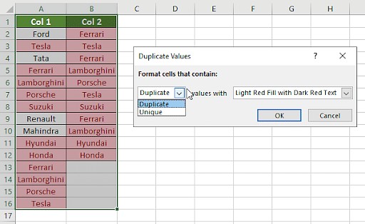
2.1. Conditional Formatting

Conditional formatting is a quick and visual way to highlight differences or similarities between two columns. Here’s how to use it:

Select the Columns: Select the two columns you want to compare.
Access Conditional Formatting: Go to the “Home” tab, click on “Conditional Formatting,” and choose “Highlight Cells Rules.”
Choose the Rule: Select “Duplicate Values” to highlight common entries or “Unique Values” to highlight differences.

Benefits: Quick visual identification of matches or differences.

Limitations: Limited to highlighting; doesn’t provide detailed comparison results.

2.2. Equals Operator (=)

The equals operator is a basic but effective way to compare cells row by row and return a TRUE or FALSE result. Follow these steps:

Create a Result Column: Add a new column where the comparison results will be displayed.
Enter the Formula: In the first cell of the result column, enter the formula =A1=B1 (assuming your data starts in row 1 of columns A and B).
Apply to All Cells: Drag the formula down to apply it to all rows.

Benefits: Simple, returns clear TRUE or FALSE results for each row.

Limitations: Doesn’t provide additional information beyond match/no match.

2.3. IF Formula

The IF formula allows you to display custom messages based on whether the values in two columns match or not.

Create a Result Column: Add a new column for the comparison results.
Enter the Formula: In the first cell of the result column, enter the formula =IF(A1=B1, "Match", "No Match").
Apply to All Cells: Drag the formula down to apply it to all rows.

Benefits: Customizable messages for matches and differences.

Limitations: Still limited to simple match/no match comparisons.

2.4. EXACT Function

The EXACT function is case-sensitive and compares two strings to determine if they are identical.

Create a Result Column: Add a new column to display the comparison results.
Enter the Formula: In the first cell of the result column, enter the formula =EXACT(A1, B1).
Apply to All Cells: Drag the formula down to apply it to all rows.

Benefits: Case-sensitive comparison for precise matching.

Limitations: Only provides TRUE or FALSE results; doesn’t handle complex logic.

2.5. VLOOKUP Function

The VLOOKUP function is used to find values in one column based on matches in another. This is particularly useful for comparing datasets where one column contains a unique identifier.

Create a Result Column: Add a new column for the comparison results.
Enter the Formula: In the first cell of the result column, enter the formula =VLOOKUP(A1, B:B, 1, FALSE). This formula looks for the value in A1 within column B.
Handle Errors: Use the IFERROR function to display a custom message when a match is not found: =IFERROR(VLOOKUP(A1, B:B, 1, FALSE), "Not Found").
Apply to All Cells: Drag the formula down to apply it to all rows.

Benefits: Can find and return related data from another column; useful for identifying missing values.

Limitations: Requires a common identifier; can be slower with large datasets.

3. Scenarios and Corresponding Methods

Different scenarios require different methods for comparing columns in Excel. Here’s a guide to help you choose the right approach:

3.1. Comparing Two Columns Row-by-Row

When you need to compare corresponding cells in two columns, use the following formulas:

=IF(A1=B1, "Match", "No Match"): Provides a simple match/no match result.
=IF(A1<>B1, "Different", "Same"): Indicates whether the values are different or the same.
=IF(EXACT(A1, B1), "Match", "No Match"): Offers a case-sensitive comparison.

3.2. Comparing Multiple Columns for Row Matches

To compare more than two columns and find complete row matches, use these formulas:

=IF(AND(A1=B1, A1=C1), "Complete Match", ""): Checks if all columns have the same value.
=IF(COUNTIF($A1:$E1, $A1)=5, "Complete Match", ""): Counts how many times the value in A1 appears across columns A to E; if it equals the number of columns, it’s a complete match.

3.3. Comparing Two Columns for Matches and Differences

To find unique values in one column that are not present in another, use these formulas:

=IF(COUNTIF($B:$B, $A1)=0, "Not in B", ""): Checks if the value in A1 is present in column B.
=IF(ISERROR(MATCH($A1, $B$1:$B$10, 0)), "Not in B", ""): Uses the MATCH function to find the value in A1 within column B and returns an error if not found.

You can also combine these for a comprehensive result:

=IF(COUNTIF($B:$B, $A1)=0, "Not in B", "Present in B"): Indicates whether the value from column A is present in column B.

3.4. Comparing Two Lists and Pulling Matching Data

To compare two lists and retrieve matching data, use the VLOOKUP, INDEX MATCH, or XLOOKUP functions:

=VLOOKUP(D1, $A$1:$B$6, 2, FALSE): Looks up the value in D1 within the range A1:B6 and returns the corresponding value from column B.
=INDEX($B$1:$B$6, MATCH($D1, $A$1:$A$6, 0)): Uses INDEX and MATCH to find the value in D1 within column A and returns the corresponding value from column B.
=XLOOKUP(D1, $A$1:$A$6, $B$1:$B$6): A more modern function that performs the same task as INDEX MATCH with simpler syntax.

3.5. Highlighting Row Matches and Differences

To highlight rows with identical values in all columns, use conditional formatting with the following formulas:

=AND($A1=$B1, $A1=$C1): Highlights rows where all three columns have the same value.
=COUNTIF($A1:$C1, $A1)=3: Highlights rows where the count of the value in A1 across columns A to C equals 3.

Alternatively, follow these steps to highlight row differences:

Select the Columns: Select the columns you want to compare.
Go to Special: On the “Home” tab, in the “Editing” group, click “Find & Select” and choose “Go To Special.”
Select Row Differences: Choose “Row Differences” and click “OK.”
Apply Formatting: The cells with different values will be selected. Change the fill color as desired.

4. Practical Examples

Let’s illustrate these methods with practical examples. Suppose you have two columns of data: Column A contains a list of product IDs, and Column B contains a list of customer IDs.

4.1. Example 1: Finding Matching Product IDs

To find which product IDs in Column A are also present in Column B, use the VLOOKUP function:

In Column C, enter the formula =IFERROR(VLOOKUP(A1, B:B, 1, FALSE), "Not Found").
Drag the formula down to apply it to all rows.

This will display the matching product ID if found in Column B or “Not Found” if it is not.

4.2. Example 2: Highlighting Differences

To visually highlight the differences between the two columns, use conditional formatting:

Select both columns.
Go to “Home” > “Conditional Formatting” > “Highlight Cells Rules” > “Duplicate Values.”
Choose “Unique” in the dropdown and select a formatting style.

This will highlight the unique product IDs in both columns, making it easy to spot the differences.

4.3. Example 3: Case-Sensitive Comparison

If you need to compare two columns with case sensitivity, use the EXACT function:

In Column C, enter the formula =EXACT(A1, B1).
Drag the formula down to apply it to all rows.

This will return TRUE if the values in A1 and B1 are exactly the same (including case) and FALSE if they are not.

5. Advanced Tips and Tricks

To further enhance your column comparison skills in Excel, consider these advanced tips:

Use Named Ranges: Define named ranges for your columns to make formulas easier to read and maintain. For example, name column A “ProductID” and column B “CustomerID.” Then, your VLOOKUP formula would look like this: =IFERROR(VLOOKUP(ProductID, CustomerID, 1, FALSE), "Not Found").
Combine Functions: Combine multiple functions to create more complex comparison logic. For instance, use the AND function with the EXACT function to perform a case-sensitive comparison of multiple columns.
Use Helper Columns: Create helper columns to perform intermediate calculations or transformations. This can simplify complex formulas and make them easier to understand.
Use Tables: Convert your data ranges into Excel tables. Tables automatically expand as you add new data, and they support structured references, making formulas more readable and maintainable.

6. Optimizing Performance for Large Datasets

When working with large datasets, performance can be a concern. Here are some tips to optimize performance when comparing columns in Excel:

Use Efficient Formulas: The VLOOKUP function can be slow with large datasets. Consider using INDEX MATCH or XLOOKUP, which are generally faster.
Avoid Volatile Functions: Volatile functions like NOW() and RAND() recalculate every time the worksheet changes, which can slow down performance. Avoid using these functions in your comparison formulas.
Disable Automatic Calculation: Temporarily disable automatic calculation while performing complex operations. To do this, go to “Formulas” > “Calculation Options” and select “Manual.” Remember to set it back to “Automatic” when you’re done.
Use Excel Power Query: For very large datasets, consider using Excel Power Query to perform the comparison. Power Query is designed to handle large amounts of data efficiently and can perform complex transformations.
Use Array Formulas: Use array formulas can sometimes provide a more efficient way to perform comparisons across multiple rows or columns. Be cautious as they can impact performance if overused.

7. Common Mistakes to Avoid

When comparing columns in Excel, avoid these common mistakes:

Ignoring Case Sensitivity: The EXACT function is case-sensitive, while the standard equals operator (=) is not. Choose the appropriate method based on your needs.
Not Handling Errors: The VLOOKUP function returns an error if a match is not found. Use the IFERROR function to handle these errors gracefully.
Using Incorrect Ranges: Double-check that your ranges are correct in your formulas. Using incorrect ranges can lead to inaccurate results.
Not Locking Ranges: When using functions like VLOOKUP, use absolute references (e.g., $A$1:$B$10) to lock the ranges. This ensures that the ranges do not change when you drag the formula down.
Forgetting Data Types: Ensure that the data types in the columns you are comparing are consistent. Comparing text to numbers can lead to unexpected results. Use the VALUE function to convert text to numbers if necessary.

8. FAQs

8.1. How can I compare two columns in Excel and return a value from a third column?

You can use the INDEX and MATCH functions together to compare two columns and return a value from a third column.

8.2. How can I compare two columns and highlight the differences?

Use conditional formatting with a formula. Select the range, go to Conditional Formatting, choose “New Rule,” select “Use a formula to determine which cells to format,” and enter a formula like =A1<>B1.

8.3. How can I compare two columns and find duplicates?

Use conditional formatting. Select the range, go to Conditional Formatting, choose “Highlight Cells Rules,” and select “Duplicate Values.”

8.4. How do I compare two lists in Excel for matches?

Use the VLOOKUP or MATCH function to check if values from one list exist in the other.

8.5. How can I compare two columns in Excel and return “Match” or “No Match”?

Use the IF function: =IF(A1=B1, “Match”, “No Match”).

8.6. Is it possible to compare two columns in Excel using the Index-Match function?

Yes, the INDEX and MATCH functions can be used for comparing columns. They are particularly useful when you need to return values from another column based on the comparison.

8.7. How to compare multiple columns in Excel?

You can compare multiple columns by using the AND function within an IF formula, or by using conditional formatting with formulas that check multiple conditions.

8.8. How do you compare two lists in Excel for matches?

You can compare two lists using functions like VLOOKUP, MATCH, or COUNTIF to find matching entries.

8.9. How do I compare two columns in Excel and highlight the duplicates?

To compare two columns and highlight duplicates, use conditional formatting with the “Duplicate Values” rule.

8.10. How to Compare Two Columns with Different Number of Rows in Excel?

To compare two columns with different number of rows, you can use formulas with IFERROR and INDEX/MATCH or VLOOKUP. This allows you to handle cases where the lookup value is not found in the shorter list.

9. Conclusion: Streamlining Data Comparison with COMPARE.EDU.VN

Comparing columns in Excel is a fundamental skill for data analysis, and mastering these techniques can significantly improve your efficiency and accuracy. Whether you’re identifying duplicates, finding unique values, or comparing datasets, the methods outlined in this guide will help you achieve your goals.

At COMPARE.EDU.VN, we understand the importance of making informed decisions based on comprehensive comparisons. That’s why we offer a wide range of resources and tools to help you compare products, services, and ideas effectively.

Ready to take your data analysis skills to the next level? Visit COMPARE.EDU.VN today to explore our comprehensive comparison guides and discover how you can make smarter, more informed decisions.

For further assistance, contact us at:

Address: 333 Comparison Plaza, Choice City, CA 90210, United States
WhatsApp: +1 (626) 555-9090
Website: COMPARE.EDU.VN

By leveraging the power of compare.edu.vn, you can unlock new insights and make better choices in all aspects of your life.