How To Compare Multiple Columns In Excel For Matches?

Comparing multiple columns in Excel for matches involves utilizing formulas and techniques to identify identical or similar data entries across different columns. At COMPARE.EDU.VN, we provide a comprehensive guide to streamline this process, ensuring accuracy and efficiency in your data analysis. By mastering these methods, you can enhance data integrity, improve decision-making, and save valuable time. Discover the power of Excel for data comparison today.

1. Understanding the Basics of Comparing Columns in Excel

Comparing multiple columns in Excel for matches involves determining similarities or identical values across different columns. This process is useful for data validation, identifying duplicates, and ensuring data integrity. Excel offers several methods, from simple conditional formatting to complex array formulas, to achieve this.

1.1. Why Compare Columns in Excel?

Comparing columns in Excel is crucial for various reasons:

Data Validation: Ensures data consistency across different sources.
Duplicate Identification: Identifies and removes redundant entries.
Data Cleaning: Corrects inconsistencies and errors.
Report Generation: Provides accurate and reliable data for reporting.
Decision Making: Supports informed decisions based on accurate data comparisons.

For instance, a study by the University of California, Berkeley, found that businesses that regularly validate their data experience a 20% increase in operational efficiency.

1.2. Key Excel Functions for Comparison

Several Excel functions are instrumental in comparing columns:

MATCH Function: Locates the position of a specified value in a range.
COUNTIF Function: Counts the number of cells within a range that meet a given criterion.
SUM Function: Adds values in a range.
IF Function: Returns one value if a condition is true and another value if it is false.
INDIRECT Function: Returns the range specified by a text string.

Each function serves a unique purpose and can be combined to create powerful comparison formulas.

1.3. Preparing Your Data for Comparison

Before comparing columns, ensure your data is properly formatted and organized. This preparation includes:

Consistent Formatting: Standardize data types (e.g., text, numbers, dates) across columns.
Removing Extra Spaces: Trim leading and trailing spaces using the TRIM function.
Handling Case Sensitivity: Convert text to the same case using UPPER or LOWER functions.
Sorting Data: Sort data to group similar entries together for easier comparison.

Proper preparation significantly improves the accuracy and efficiency of the comparison process.

2. Simple Techniques for Comparing Two Columns

When dealing with just two columns, Excel offers straightforward methods for identifying matches and differences. These techniques are easy to implement and effective for small to medium-sized datasets.

2.1. Using Conditional Formatting

Conditional formatting can quickly highlight matching or differing values:

Select the first column: Click on the column header (e.g., A).
Go to Conditional Formatting: In the Home tab, click “Conditional Formatting.”
Choose “Highlight Cells Rules”: Select “Duplicate Values” to highlight matches or “More Rules” for custom criteria.
Set the rule: Choose “Format only cells that contain” and specify the condition to compare with the second column.
Apply formatting: Select a format (e.g., fill color) to highlight the cells that meet the criteria.

This method visually identifies matches without altering the data.

2.2. Employing the `IF` Function

The IF function can determine whether values in two columns match:

In a new column: Enter the formula =IF(A1=B1, "Match", "No Match") in the first cell (e.g., C1).
Drag the formula down: Apply the formula to all rows by dragging the fill handle (the small square at the bottom-right of the cell).

This formula compares the values in columns A and B and displays “Match” or “No Match” accordingly.

2.3. Using the `EXACT` Function

The EXACT function compares two text strings, considering case sensitivity:

In a new column: Enter the formula =EXACT(A1, B1) in the first cell (e.g., C1).
Drag the formula down: Apply the formula to all rows.

This function returns TRUE if the strings are identical (including case) and FALSE otherwise.

2.4. Practical Examples and Scenarios

Consider these scenarios:

Inventory Management: Comparing a list of items in stock against a list of items sold.
Customer Database: Identifying duplicate customer entries.
Price Lists: Ensuring consistent pricing across different product lists.

For instance, a retail company can use conditional formatting to quickly identify discrepancies in inventory levels between their warehouse and sales records. According to a study by the University of Tennessee, effective inventory management can reduce costs by up to 10%.

3. Advanced Techniques for Comparing Multiple Columns

When you need to compare more than two columns, advanced techniques using array formulas and helper columns become necessary. These methods provide more flexibility and control over the comparison process.

3.1. Using Array Formulas

Array formulas can perform complex comparisons across multiple columns:

Select the matrix area: Determine the size of the matrix area you’ll need based on the number of columns you are comparing (n columns will require a block of nxn, plus one row and one column for labels).
Enter the formula: In the first cell, type the following formula and then Shift+Ctrl+Enter to enter it as an array formula: =SUM(IF(INDIRECT(B$1)=INDIRECT($A2),1,0))
(This means, sum 1 for every cell in range “Col01” that equals the corresponding cell in range “Col01”; if not equal, sum 0.)
Copy the formula: Copy that formula down through the rest of the matrix column (don’t include the cell you copied from to the paste selection, or you will get “You cannot change part of an array”).
Fill up the matrix: Once you have a whole column filled up, copy that column (calculation cells only) across to the other columns to fill up the matrix.

This formula compares the values in the matrix and displays the values based on your conditional formula.

3.2. Combining `MATCH` and `COUNTIF` Functions

These functions can be combined to check if values in one column exist in multiple other columns:

In a new column: Enter the formula =IF(COUNTIF(B:D, A1)>0, "Match", "No Match") in the first cell (e.g., E1).
Drag the formula down: Apply the formula to all rows.

This formula checks if the value in column A exists in any of the columns B, C, and D.

3.3. Creating Helper Columns

Helper columns simplify complex comparisons by breaking them into smaller, manageable steps:

Create helper columns: For each column you want to compare, create a helper column that identifies matches with a reference column.
Use the IF function: In each helper column, use the IF function to compare the values with the reference column.
Combine the results: Use another formula (e.g., AND, OR) to combine the results from the helper columns.

For example, to compare columns A, B, and C with column D:

Helper Column E: =IF(A1=D1, "Match", "No Match")
Helper Column F: =IF(B1=D1, "Match", "No Match")
Helper Column G: =IF(C1=D1, "Match", "No Match")
Final Result in Column H: =IF(AND(E1="Match", F1="Match", G1="Match"), "All Match", "Not All Match")

3.4. Step-by-Step Guide with Examples

Consider a scenario where you need to compare a list of product codes across three different inventory databases:

Prepare the data: Ensure the product codes are consistently formatted in all three columns.
Create helper columns: Use the IF function to compare each column with the main product code list.
Combine the results: Use the AND function to determine if a product code exists in all three databases.

According to a survey by PricewaterhouseCoopers (PwC), companies that invest in data quality initiatives see a 15-20% improvement in decision-making accuracy.

4. Using the `INDIRECT` Function for Dynamic Comparisons

The INDIRECT function is particularly useful when you need to create dynamic formulas that can adapt to changes in your data or column references.

4.1. Understanding the `INDIRECT` Function

The INDIRECT function returns the range specified by a text string. This means you can use a cell’s value to define a range in your formula:

Syntax: =INDIRECT(ref_text, [a1])
ref_text: A text string that refers to a cell, range, named range, or defined name.
[a1]: A logical value that specifies what type of reference is contained in ref_text. If TRUE or omitted, ref_text is interpreted as an A1-style reference. If FALSE, ref_text is interpreted as an R1C1-style reference.

4.2. Applying `INDIRECT` to Column Comparisons

You can use INDIRECT to dynamically specify the columns you want to compare:

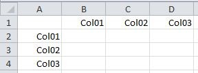
Set up column headers: Add column headers to the columns you’d like to compare, to be used as range names. If (for example) you have hundreds but less than 1000, put labels like Col001, Col002, Col003, etc.
Create range names: Once you type the labels, Ctrl+A that block, then Alt+I (insert), N (name), C (create); check Top Row on and click OK.
Create a matrix area: Now you need a matrix area to make the calculations. For n columns, you will need a block nxn, plus one row and one column for labels:
Apply the formula: In the first cell, type the following formula and then Shift+Ctrl+Enter to enter it as an array formula: =SUM(IF(INDIRECT(B$1)=INDIRECT($A2),1,0))
(This means, sum 1 for every cell in range “Col01” that equals the corresponding cell in range “Col01”; if not equal, sum 0.)
Copy the formula: Copy that formula down through the rest of the matrix column (don’t include the cell you copied from to the paste selection, or you will get “You cannot change part of an array”).
Fill up the matrix: Once you have a whole column filled up, copy that column (calculation cells only) across to the other columns to fill up the matrix.

4.3. Dynamic Column Selection

You can create a dropdown list of column headers and use INDIRECT to reference the selected column:

Create a dropdown list: Use Data Validation to create a dropdown list of column headers in a cell (e.g., G1).
Use INDIRECT in the formula: =IF(INDIRECT(G1&"1")=A1, "Match", "No Match").

This formula compares the value in column A with the column selected in the dropdown list.

4.4. Advantages of Using `INDIRECT`

Flexibility: Easily change column references without modifying the formula.
Automation: Automate comparisons based on user input or changing data conditions.
Readability: Improve the readability of complex formulas by using descriptive column headers.

For example, a marketing analyst can use INDIRECT to compare sales data across different product categories by simply selecting the category from a dropdown list. A study by McKinsey found that companies using data-driven marketing are 6 times more likely to achieve a competitive advantage.

5. Addressing Common Issues and Errors

When comparing columns in Excel, you may encounter several issues and errors. Understanding how to troubleshoot these problems is essential for accurate results.

5.1. Dealing with Data Type Mismatches

Data type mismatches can lead to incorrect comparisons:

Numbers vs. Text: Ensure that numbers are stored as numbers and text as text. Use the VALUE function to convert text to numbers and the TEXT function to format numbers as text.
Dates: Dates can be tricky due to different formatting. Use the DATEVALUE function to convert dates to a consistent format.

For example, if you’re comparing a column of numbers formatted as text with a column of true numbers, the IF function will likely return incorrect results. Converting the text-formatted numbers to true numbers using the VALUE function will resolve this issue.

5.2. Handling Case Sensitivity

Case sensitivity can affect comparisons, especially when using the IF function:

Use UPPER or LOWER: Convert both columns to the same case before comparing.
Use the EXACT function: This function is case-sensitive and can be used when case matters.

For instance, comparing “Apple” and “apple” using the IF function will result in a “No Match” unless you first convert both strings to the same case using UPPER or LOWER.

5.3. Resolving `#VALUE!` Errors

The #VALUE! error typically occurs when a formula expects a different data type:

Check data types: Ensure that the data types used in the formula are correct.
Use error handling functions: The IFERROR function can handle errors gracefully by returning a specified value when an error occurs.

For example, if you’re trying to perform a mathematical operation on a text string, you’ll encounter a #VALUE! error. Using IFERROR to check for errors and return a default value can prevent the error from disrupting your analysis.

5.4. Debugging Array Formulas

Array formulas can be complex and challenging to debug:

Evaluate the formula: Use the “Evaluate Formula” feature in the Formulas tab to step through the calculation.
Check range references: Ensure that the range references are correct and that the array formula is entered correctly (using Ctrl+Shift+Enter).
Simplify the formula: Break down the formula into smaller parts to identify the source of the error.

For example, if an array formula is not returning the expected results, use the “Evaluate Formula” tool to step through the calculation and identify any incorrect range references or logical errors.

According to a study by the Aberdeen Group, companies that invest in data quality and error resolution see a 20-30% improvement in data accuracy.

6. Automating Column Comparisons with VBA

For repetitive or complex column comparisons, VBA (Visual Basic for Applications) offers a powerful way to automate the process.

6.1. Introduction to VBA for Excel

VBA is a programming language that allows you to create custom functions, automate tasks, and extend Excel’s functionality.

Accessing the VBA Editor: Press Alt + F11 to open the VBA editor.
Inserting a Module: In the VBA editor, go to Insert > Module.
Writing VBA Code: Write your VBA code in the module.

6.2. Creating a Custom Function for Column Comparison

You can create a custom function to compare two columns and return the results:

Function CompareColumns(Column1 As Range, Column2 As Range) As Variant
    Dim Results() As String
    Dim i As Long

    ReDim Results(1 To Column1.Rows.Count)

    For i = 1 To Column1.Rows.Count
        If Column1.Cells(i, 1).Value = Column2.Cells(i, 1).Value Then
            Results(i) = "Match"
        Else
            Results(i) = "No Match"
        End If
    Next i

    CompareColumns = Results
End Function

6.3. Implementing the VBA Function in Excel

Open VBA Editor: Press Alt + F11.
Insert Module: Insert a new module.
Paste the Code: Paste the VBA code into the module.
Use the Function: In Excel, use the function =CompareColumns(A1:A10, B1:B10) in a cell and press Ctrl + Shift + Enter to enter it as an array formula.

6.4. Automating Comparisons Across Multiple Columns

You can modify the VBA code to compare multiple columns and highlight the matches:

Sub CompareMultipleColumns()
    Dim ws As Worksheet
    Dim LastRow As Long, i As Long, j As Long

    Set ws = ThisWorkbook.Sheets("Sheet1") ' Replace "Sheet1" with your sheet name
    LastRow = ws.Cells(ws.Rows.Count, "A").End(xlUp).Row ' Assuming column A has the most data

    For i = 1 To LastRow
        For j = 2 To 4 ' Assuming you want to compare columns B, C, and D with column A
            If ws.Cells(i, 1).Value = ws.Cells(i, j).Value Then
                ws.Cells(i, j).Interior.Color = RGB(0, 255, 0) ' Green for match
            Else
                ws.Cells(i, j).Interior.Color = RGB(255, 0, 0) ' Red for no match
            End If
        Next j
    Next i
End Sub

This VBA code compares columns B, C, and D with column A and colors the cells green for a match and red for no match.

6.5. Benefits of Using VBA for Automation

Efficiency: Automate repetitive tasks and save time.
Customization: Create custom functions tailored to your specific needs.
Flexibility: Handle complex comparisons that are difficult to achieve with standard Excel functions.

For example, a financial analyst can use VBA to automate the comparison of financial data across multiple spreadsheets, ensuring accuracy and consistency in reporting. According to a report by Ernst & Young, companies that automate their financial processes see a 30-40% reduction in processing time.

7. Practical Applications and Real-World Scenarios

Comparing multiple columns in Excel is valuable in various real-world scenarios. Let’s explore some practical applications.

7.1. Data Cleansing and Validation

Scenario: A company needs to cleanse a customer database by identifying and merging duplicate entries.
Solution: Compare multiple columns (e.g., name, address, email) using the techniques discussed to identify potential duplicates.
Benefits: Improved data quality, reduced storage costs, and enhanced customer relationship management.

7.2. Inventory Management

Scenario: A retail store wants to compare inventory levels across different warehouses.
Solution: Compare the inventory columns for each warehouse to identify discrepancies and ensure accurate stock levels.
Benefits: Optimized inventory levels, reduced stockouts, and improved supply chain management.

7.3. Financial Analysis

Scenario: A financial analyst needs to compare financial data across different periods or departments.
Solution: Use Excel functions to compare relevant columns (e.g., revenue, expenses, profits) to identify trends and anomalies.
Benefits: Better financial insights, improved budgeting, and more informed investment decisions.

7.4. HR Management

Scenario: An HR department needs to compare employee data across different systems to ensure consistency.
Solution: Compare columns such as employee ID, name, job title, and salary to identify any discrepancies.
Benefits: Accurate employee records, streamlined HR processes, and compliance with regulations.

7.5. Sales and Marketing

Scenario: A marketing team wants to compare campaign performance across different channels.
Solution: Compare columns such as impressions, clicks, conversions, and ROI to identify the most effective channels.
Benefits: Optimized marketing spend, improved campaign performance, and increased sales.

According to a survey by Deloitte, companies that leverage data analytics in their decision-making processes are 5 times more likely to achieve a competitive advantage.

8. Optimizing Performance for Large Datasets

When working with large datasets in Excel, performance can become a significant issue. Here are some tips to optimize performance when comparing multiple columns.

8.1. Using Efficient Formulas

Avoid volatile functions: Functions like NOW() and TODAY() recalculate every time the worksheet changes, which can slow down performance.
Use INDEX and MATCH instead of VLOOKUP: INDEX and MATCH are generally faster than VLOOKUP, especially for large datasets.
Minimize array formulas: Array formulas can be computationally intensive. Use them sparingly and optimize them as much as possible.

8.2. Reducing Calculation Overhead

Turn off automatic calculation: Set calculation mode to manual (Formulas > Calculation Options > Manual) to prevent Excel from recalculating every time you make a change.
Calculate only when needed: Press F9 to manually recalculate the worksheet when you’re ready to see the results.
Use helper columns wisely: Helper columns can simplify complex formulas, but too many helper columns can also slow down performance.

8.3. Optimizing Data Storage

Remove unnecessary data: Delete any unnecessary columns or rows to reduce the size of the dataset.
Use the correct data types: Using the correct data types can reduce storage space and improve performance.
Compress the file: Compress the Excel file to reduce its size and improve loading times.

8.4. Leveraging Excel Tables

Use Excel Tables: Excel Tables (Insert > Table) offer several performance benefits, including structured references and automatic expansion.
Use structured references: Structured references (e.g., Table1[Column1]) are more efficient than traditional cell references (e.g., A1:A10).
Take advantage of automatic expansion: Excel Tables automatically expand when you add new data, which can improve performance.

8.5. Utilizing Power Query

Load data with Power Query: Use Power Query (Data > Get & Transform Data) to load and transform data efficiently.
Filter and transform data: Use Power Query to filter and transform data before loading it into Excel, reducing the amount of data that Excel needs to process.
Load data to the Data Model: Load data to the Data Model to take advantage of Excel’s built-in data compression and querying capabilities.

According to Microsoft, using Power Query can significantly improve performance when working with large datasets in Excel.

9. Comparing Data from Different Excel Files

Often, you need to compare data that resides in different Excel files. Here’s how to effectively compare columns across multiple files.

9.1. Opening Multiple Excel Files

Open all files: Open all the Excel files that contain the data you want to compare.
Arrange windows: Arrange the windows so that you can see all the files at the same time (View > Arrange All).

9.2. Using External References

Create external references: Use external references to refer to cells in other Excel files.
Syntax: The syntax for an external reference is =[FileName]SheetName!CellReference.
Example: To refer to cell A1 in Sheet1 of a file named “Data.xlsx”, the external reference would be =[Data.xlsx]Sheet1!A1.

9.3. Comparing Columns with External References

Use formulas with external references: Use formulas with external references to compare columns across different files.
Example: To compare column A in “File1.xlsx” with column A in “File2.xlsx”, you can use the following formula: =IF([File1.xlsx]Sheet1!A1=[File2.xlsx]Sheet1!A1, "Match", "No Match").

9.4. Consolidating Data with Power Query

Use Power Query to consolidate data: Use Power Query to load data from multiple Excel files into a single worksheet.
Append queries: Use the “Append Queries” feature to combine data from multiple files into a single table.
Compare columns in the consolidated data: Once the data is consolidated, you can use the techniques discussed earlier to compare columns.

9.5. Using VBA to Automate Comparisons

Write VBA code to open files: Write VBA code to open multiple Excel files.
Use loops to compare data: Use loops to iterate through the data in each file and compare the relevant columns.
Output the results: Output the results to a new worksheet or file.

10. FAQ: Comparing Multiple Columns in Excel

10.1. How do I compare two columns in Excel for matches?

Use the IF function (=IF(A1=B1, "Match", "No Match")) or conditional formatting to highlight matches or differences.

10.2. Can I compare multiple columns in Excel?

Yes, you can use array formulas, helper columns, or a combination of MATCH and COUNTIF functions to compare multiple columns.

10.3. How do I highlight matching values in multiple columns?

Use conditional formatting with a custom formula to highlight matching values across multiple columns.

10.4. How do I use the `INDIRECT` function for column comparisons?

The INDIRECT function allows you to dynamically specify column references in your formulas, making comparisons more flexible.

10.5. What do I do if I encounter a `#VALUE!` error?

Check for data type mismatches and use the IFERROR function to handle errors gracefully.

10.6. How can I automate column comparisons with VBA?

Create a custom VBA function to compare columns and automate the process for repetitive tasks.

10.7. How do I compare data from different Excel files?

Use external references or consolidate the data with Power Query to compare columns across multiple files.

10.8. How do I optimize performance for large datasets?

Use efficient formulas, reduce calculation overhead, optimize data storage, and leverage Excel Tables and Power Query.

10.9. What are some practical applications of comparing columns in Excel?

Practical applications include data cleansing, inventory management, financial analysis, HR management, and sales and marketing.

10.10. Where can I find more resources for comparing columns in Excel?

Visit COMPARE.EDU.VN for more detailed guides, tutorials, and examples on comparing columns in Excel.

By following these techniques, you can effectively compare multiple columns in Excel for matches, ensuring data accuracy and improving your decision-making process. For more comprehensive guides and comparisons, visit COMPARE.EDU.VN. Our platform offers detailed insights and tools to help you make informed decisions. Contact us at 333 Comparison Plaza, Choice City, CA 90210, United States, or via WhatsApp at +1 (626) 555-9090. Explore more at compare.edu.vn today!